Demand the impossible: rigorous database benchmarking
29 Dec 20230. Table of content
- Introduction
- PostgreSQL
- Statistics
- Even more smooth transition to statistics
- A century old problem
- Big problem in CS
- How many runs do we need?
- Randomized testing
- Time average or ensemble average?
- Summary
- References
1. Introduction
Everyone knows benchmarking is hard (and writing about benchmarking is double as hard), but have you ever asked “why”? What makes benchmarking, and performance evaluation in general, so error-prone, so complicated to get right and so easy to screw up? Those are not new questions, but there seem to be no definitive answer, and for databases things are even more grim – yet we could speculate, hoping that our speculation can help us learn something along the way. I don’t think you would read anything new below, in fact many things I’m going to talk about are rather obvious – but the process of bringing everything together and thinking about the topic is valuable by itself.
There could be at least few reasons why it’s so easy to fail trying to understand performance of a database system, and they usually have something to do with the inherent duality:
- It’s necessary to combine expertise from both the domain specific area and general analytics expertise.
- One have to take into account both known and unknown factors.
- Establishing a comprehensive mental model of a database is surprisingly hard and could be counter-intuitive at times.
1.1 Common vs particular
We would refer to the expertise from a domain specific area as a “particular knowledge”, for the purposes of this article it means PostgreSQL details. The general expertise is going under a “common knowledge”, mostly meaning statistics and data analysis. We’re talking here about combining common knowledge, something that could be applied in many situations, and particular knowledge, which is specific to an area we’re exploring. Those two type of expertise are often orthogonal and take extra efforts to combine.
1.2 Known vs unknown
More than once a proper benchmark was failed due to an obscure effect not being taken care of. This even goes beyond obvious known/unknown classification, and we usually have following:
-
Known knowns, e.g. we know
max_wal_sizeparameter plays a significant role in PostgreSQL performance. -
Known unknowns, e.g. we know
max_wal_sizeis important, but have no idea what is the optimal value. -
Unknown unknowns, e.g. we have no idea that we run the database on a buggy Linux Kernel version, where buffered IO in a cgroup is slow due to wrong memory pressure calculation and constant page reclaiming.
-
Intrinsic noise, e.g. we run the database on a disk with particularly volatile latencies.
1.3 Database model
Everyone has a different way of thinking about databases, and what we’re going to talk about in this section is only one particular example I find useful. The idea is to view a database as a complex system that could be described as a function on the phase space, something like this:
The phase space plot of the Lorenz attractor, [1]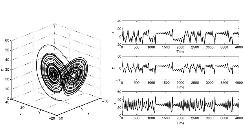
On the graph above you can see the famous Lorenz attractor, and that is exactly what I have in mind. Looking at those nice and smooth trajectories, it’s coming as a surprise what kind of graphs you get, when projecting it to only one dimension (somehow reminiscent of real latency plots). You may ask, what are the dimensions of our database model? Well, that’s where things get a bit scary – there are a lot of dimensions, which could be roughly grouped into following categories:
- Database parameters: all configuration knobs obviously affect the system performance one way or another.
- Hardware resources: another obvious part, the database is going to perform differently if you give it more memory or CPU cores.
- Workload parameters: what exactly load we apply is important as well, the results are going to be different if we do one transaction per second vs if we hit it with thousands of tps.
- Performance results: surprisingly, the output of our system is also a part of the model. Note, that in this article we’re talking about performance, but the very same approach could be made for anything else, e.g. one can build a model describing the database availability to verify HA properties.
Besides the fact that we got a lot of dimensions here, some of them are not even deterministic (mostly out of the latest category) and could be defined only as random variables with certain probability distribution, which would lead us later on the dark path of statistics. At the end we’re of course trying to simplify things and usually, at the risk of loosing high level interaction between parameters, we work with much smaller models.
A simplified (artificial) model showing
dependency between buffer size, amount of incoming queries and the
resulting latency. 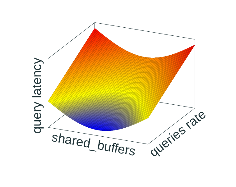
1.4 Smooth transition away from hand waving
Having said all that, lets see if there are any actual facts to back it up. We will try to use ideas described above as a framework to answer the following: how to not blow up your PostgreSQL benchmark? In fact, it’s most likely going to be more generic than that, and certain bits could be applied much broader. Nevertheless, PostgreSQL is going to be our reference point in this ever-changing world.
To make it more down to earth, imagine we’re trying to understand how database performs under certain conditions. We’ve run a benchmark and got some numbers:
latency average = 0.011 ms
latency stddev = 0.002 ms
tps = 89357.630697 (without initial connection time)
They’re filed in a report, everyone is happy. Now, few weeks later we try to repeat the same test again, and suddenly…
latency average = 0.014 ms
latency stddev = 0.023 ms
tps = 67107.536620 (without initial connection time)
…oh, crap, the numbers are quite different. It’s an unpleasant situation to be in, and we have to figure out two things: why the numbers are different, and how to prevent this type of situations in the future.
2. PostgreSQL
PostgreSQL is a great database that works most of the time, but, as any database, it’s a complex system with many moving parts – which makes it easier to miss something when it comes to performance. Unfortunately, the only way to handle this is to know where to look at, when things go south.
2.1 Misconfiguration
Most of the time the problem would be a simple misconfiguration, i.e. you forgot to tune some important parameter, and the database was behaving in an unexpected way.
It's easy to get lost in configuration
If that happened, we got an excuse – there are damn many various knobs one can configure! The community is fighting against growing number of configuration options, the idea is that it’s much better to make PostgreSQL smarter when possible. But despite that, the amount of configurable knobs is still going up, extrapolating from the graph below the growth is still linear. And don’t let me start talking about non-public configurations.
It's easy to get lost in configuration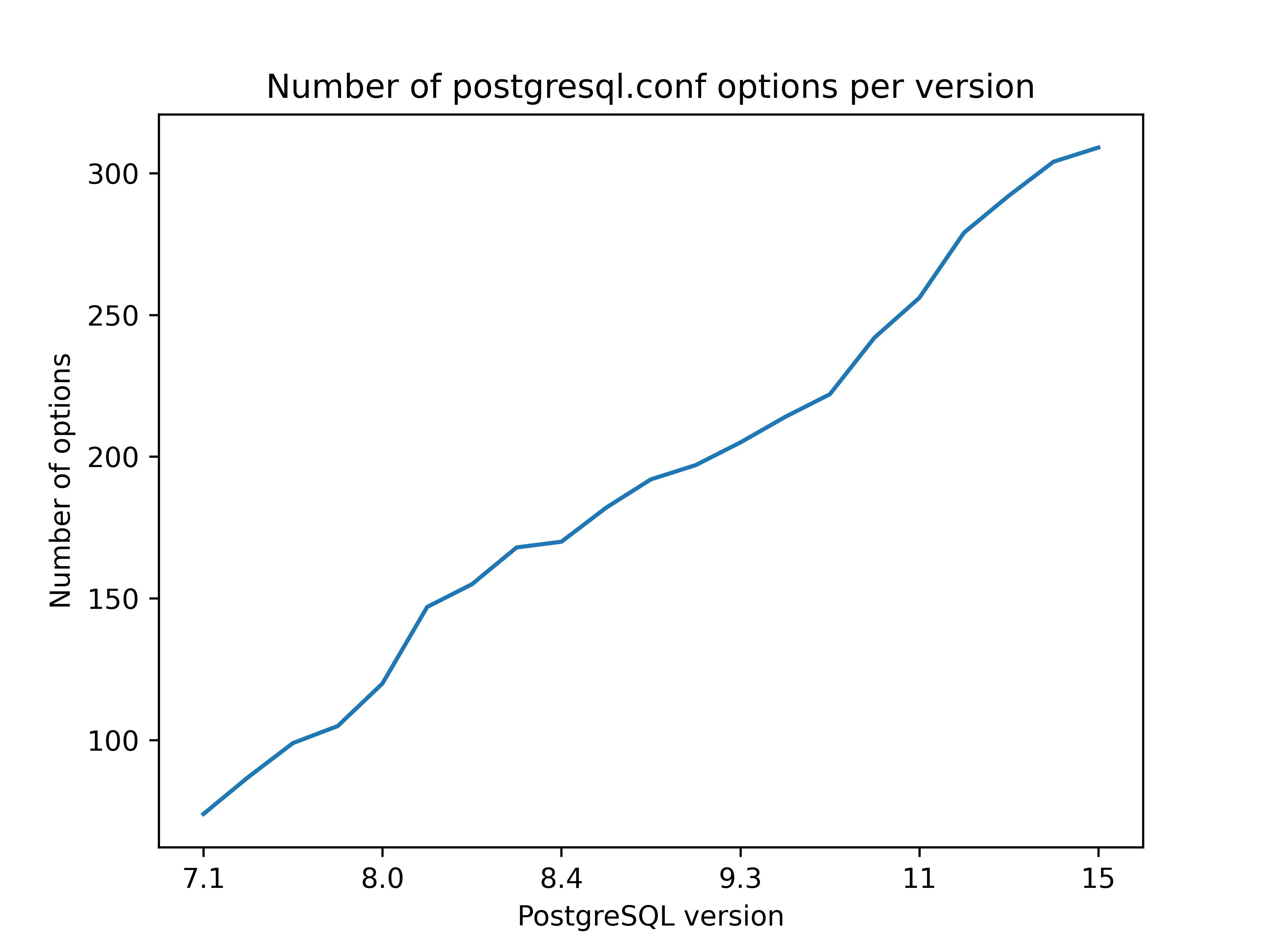
Fortunately for us, things are not so bad, and despite millions of various subtleties there is only a handful of parameters one have to know to be on the safe side most of the time. Usually the list looks something like this:
    shared_buffers
    max_wal_size
    work_mem
    checkpoint_timeout
    checkpoint_completion_target
    wal_writer_flush_after
    checkpoint_flush_after
    [...]
Of course, depending on the situation the importance of parameters could be different, but nevertheless there is a subset of all the options that can give you some confidence. How large is this subset? One interesting white paper [2], about using ML for database tuning, has this to say about the topic:
[…] one can achieve a substantial portion of the performance gain from configurations generated by ML-based tuning algorithms by setting two knobs according to the DBMS’s documentation. These two knobs control the amount of RAM for the buffer pool cache and the size of the redo log file on disk.
We can’t answer the question “how large is the subset of most important
performance configuration options” generally, but at least in the context of
automatically tuned database it’s quite modest and consist of shared_buffers
and max_wal_size. Coincidently, if we take a look at how the Postgres95 1.01
distribution looked like (it’s still in the PostgreSQL git repository), one of
the few performance relevant options that were available back then was the size
of buffer pool (there was no WAL logging yet):
   /* ----------------
    *  specify the size of buffer pool
    * ----------------
    */
   NBuffers = atoi(optarg);
Identifying relevant options is good, but figuring out what values should we use is still an open question. In fact, it’s your responsibility as a person conducting the benchmark to adjust values based on the result, sort of feedback control loop. The usual rule of thumb is that, not taking into account higher level interactions, too small or too large value are performing worse than the sweet spot in the middle (but it doesn’t help much, as we still have to identify what is the range of too small and too large).
As a side note, I’ve heard many times when people were resisting to do this type of feedback tuning, claiming they want to test the system under the real conditions. It’s a reasonable request, but clear performance results not obscured by the noise are not the only goal – often it’s hard to imagine happy users, when the database performance is frustratingly variable. Which means the optimal approach might as well include the feedback tuning.
2.2 Choose the right scale
You probably have noticed that in the motivating example at the beginning (the one with latencies from pgbench) the queries are rather fast. It’s a good example of the old maxima – understand what you benchmark. Or to be more precise, get a clear picture of what is the scale of the impact you’re expecting to see.
Sometimes it could be about a subtle development patch, a change in the transaction processing hot path, and the effect we’re looking for is going to be visible with large number of fast transactions. At the same time this effect could be easily hidden from us if something will drag the database in the other direction, e.g. it will start allocating new WAL files getting into all the troubles with fs journaling and performing IO. Thus, we have to prevent database from doing slow latency operations and configure correspondingly.
Some other times the goal would be to compare two data schemas overall, and we would like to get a holistic picture with all the bells and whistles running inside the database. In this case we do not care about how the database will handle millions of fast transactions, in fact we probably would use our own custom workload generator to simulate the expected workload. There is still some tuning to do, as we need to achieve stable enough results, see the previous section.
The idea is simple to explain, but hard to implement – we would like to
configure the database in such a way, that the effect interesting to us is
going to be amplified, while everything else will be downplayed. To achieve
that we need visibility into what’s going on: collect all available
statistics, enable all the necessary
logging, probably also use some static and dynamic
instrumentation with whatever tool you prefer to use (perf, bcc,
bpftrace, etc). The plan is usually to prepare an initial configuration, run
the test, and if the results differ from expectations or the variance is higher
that the effect we would like to observe – then search through the metrics,
trying to understand what the database is doing above of what you’ve asked it
to do. It could be as easy as looking at the logs to see that the database is
choking on vacuum because it’s misconfigured, or seeing too many WALSync wait
events because NVMe device trimming kicked in.
2.3 Time dimension
While we’re talking about vacuum, here is the thing – it’s important to appreciate the time dimension of our test, since we’re dealing with a stateful system and there are a lot of time-dependent parameters. Periodic checkpointing of the data, autovacuum, replicas not catching up with the load, data bloat, you name it. This question is closely intertwined with those mentioned in the previous sections: you have to monitor all of that; even just for autovacuum there is a bunch of parameters you can tune:
# the default configuration
autovacuum_naptime = 1min
autovacuum_vacuum_threshold = 50
autovacuum_vacuum_insert_threshold = 1000
autovacuum_vacuum_scale_factor = 0.2
autovacuum_vacuum_insert_scale_factor = 0.2
autovacuum_vacuum_cost_delay = 2ms
autovacuum_vacuum_cost_limit = -1
All what I’ve said so far is essentially a repetition, but still I find it’s important to emphasize often overlooked topic of time. Obviously it’s challenging to run a benchmark to cover the time dimension fully, and the range could vary from minutes to days! Yet at least it’s better to understand which part of time-related behaviour did you observe, as it may give you an impression how it will all work in the long run.
2.4 It’s not the database
Unfortunately, no matter how much we try, PostgreSQL cannot run in the vacuum. In fact, in the modern days of cloud services, virtualization and containerization, it’s more likely to be similar to the recursive lake Sidihoni in North Sumatra, which is a lake on an island in a lake on an island. This situation, when many isolation layers are stacked one on top of another, has a very unpopular consequence – the performance problem we’re looking for could be not in the database.
Essentially it’s nothing new at this point, just the scope is becoming larger. Not only we have to keep an eye on the database configuration, it’s also beneficial to touch at least most important knobs of your kernel, filesystem, VM, etc. At the very least it makes sense how filesystem cache and disks are configured:
vm.nr_hugepages
vm.dirty_background_bytes
vm.dirty_bytes
block/<dev>/queue/read_ahead_kb
block/<dev>/queue/scheduler
Another side of the problem is the noise, which is usually coming from the underlying components. Depending on the scale, you may want to look at usual suspects:
- CPU/NUMA migrations, p-state, frequency scaling
- Files creation, NVMe trim, IO throttling from Linux
- Noisy neighbours, virtualized infrastructure, simply faulty hardware on the cloud provider side (yes, it happens).
As an interesting example, not so long ago I was struggling with one in-memory experiment, where the latencies were mysteriously raising up after certain fixed time interval. It looked like this:
Query latency for the in-memory insert workload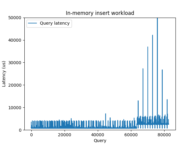
Looks pretty weird for a dataset that completely fits into the memory. I was
trying to figure out what is responsible for this latency bump, configured all
the PostgreSQL things I could think of – but without any visible impact.
Eventually I’ve tried to measure pure fsync latency with bpftrace, and
surprisingly got a two modal distribution:
@nsecs:
[1K, 2K)         1 |                                                    |
[2K, 4K)         0 |                                                    |
[4K, 8K)         0 |                                                    |
[8K, 16K)        0 |                                                    |
[16K, 32K)       0 |                                                    |
[32K, 64K)       8 |                                                    |
[64K, 128K)      0 |                                                    |
[128K, 256K)     2 |                                                    |
[256K, 512K)     0 |                                                    |
[512K, 1M)   63599 |@@@@@@@@@@@@@@@@@@@@@@@@@@@@@@@@@@@@@@@@@@@@@@@@@@@@|
[1M, 2M)       426 |                                                    |
[2M, 4M)     18626 |@@@@@@@@@@@@@@@                                     |
[4M, 8M)       110 |                                                    |
[8M, 16M)       20 |                                                    |
[16M, 32M)       3 |                                                    |
[32M, 64M)       4 |                                                    |
Plotting fsync and query latencies side by side proved the correlation and that the reason for this latency bump was under the database.
Same as the previous one, but now with fsync latency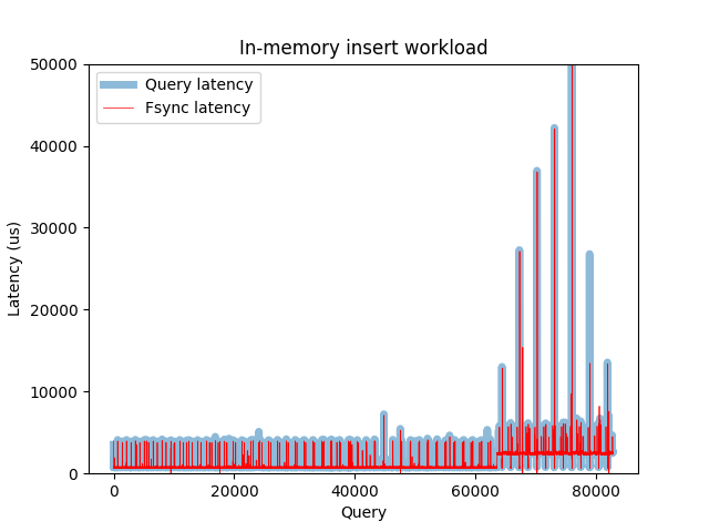
2.5 Load generator
It may come as a surprise, but the load generator is as important as the tested subject itself. If you got a misconfigured generator, you will probably get misleading results as well. Fortunately we’ve got many options to chose from:
- Benchbase (former OLTPBench)
- Sysbench (more general benchmarking tool)
- YCSB (for “key-value” loads)
- HammerDB (cross-database tool from TPC)
- pgbench (out of the box benchmarking tool for PostgreSQL)
- Replicated live workload (the most cumbersome, but rewarding option)
Those tools are great, but they still leave room for mistakes. For example if
misconfigured, the benchmarking tool could be a bottleneck on its own, leading
to misleading results. Even how much work the benchmarking tool is doing could
affect the outcome – remember our motivational example at the beginning of the
article? The mystery is simple, we ran pgbench two times, one only with
aggregate statistics reporting, another with individual latency logging (and
hence much more things for it to do).
But there is even more subtle issue lurking behind benchmarking tooling. If we think about “server <-> load generator” system in the context of queueing theory, accepting some necessary simplification, it’s usually described as an “open system” [3], meaning that new queries arrive independently of queries completion and are governed by an arrival rate exclusively.
An open system [3]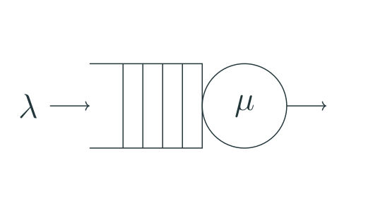
But what usually happens when we use a workload generator is different – it either tries to keep the same number of queries in fly, or sends queries as quickly as possible sequentially (at least within every parallel workers), a new one comes in after the previous is finished. This approach is called a “closed system” in queueing theory, and unfortunately has different properties, especially when it comes to tail latencies.
A closed system [3]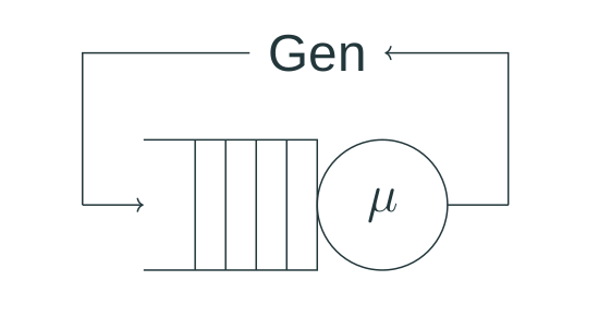
It’s not the end of the world, and workload generators that use this approach still provide valuable information. But it’s important to understand the difference and realize that under the real workload p99 can look worse than in the experiments. At the same time, as far as I can tell, at least Benchbase allows to use the first approach as well, generating arriving queries using Poisson distribution with a specified rate.
3. Statistics
3.1 Even more smooth transition to statistics
Despite having spent a lot of words, we’ve barely scratched the surface of “particular” knowledge for PostgreSQL. But even if we assume for a moment that we take everything into account, there is still plenty opportunities to interpret the data wrong, or get fooled by noise and irrelevant correlations. For example, the authors of this paper [4] show that even experts often make an error mixing up precision of statistical estimation (like standard error) with the result variability (like standard deviation) – leading to much confusion and wrong interpretation of the data. Thus, we have to learn few tricks from statistics.
3.2 A century old problem
Let’s start with an interesting fact – what we discuss here is not at all a new problem. On the contrary, benchmarking using various statistic methods has been a thing in natural sciences for at least one century, and scientists are doing essentially the same what we do here: change certain system in a controlled way and compare the results before and after. Most of the time it’s about experimenting what type of fertilizer is better for tomatoes, or what is the most optimal way to produce a certain chemical reaction. Still it’s not able to conceal the real goal – conquering and rule the world using statistics.
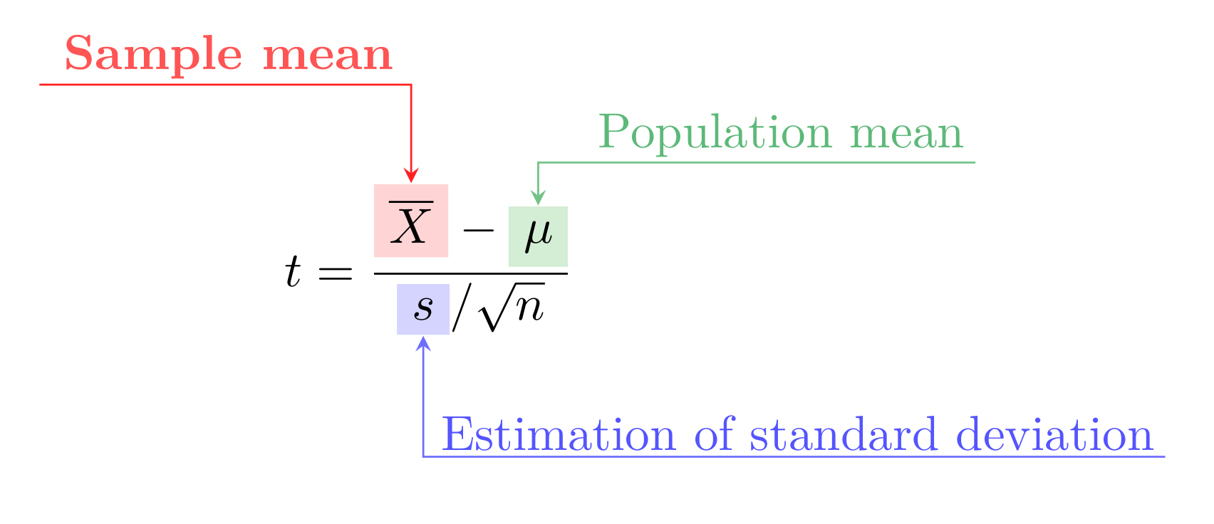
For example, the well known “Student’s t-distribution” got its name from W. S. Gosset, who first published an article about it in 1908 [5] (the author was interested in determining the quality of raw material at Guiness Brewery):
Now any series of experiments is only of value in so far as it enables us to form a judgement as to the statistical constants of the population to which the experiment belong.
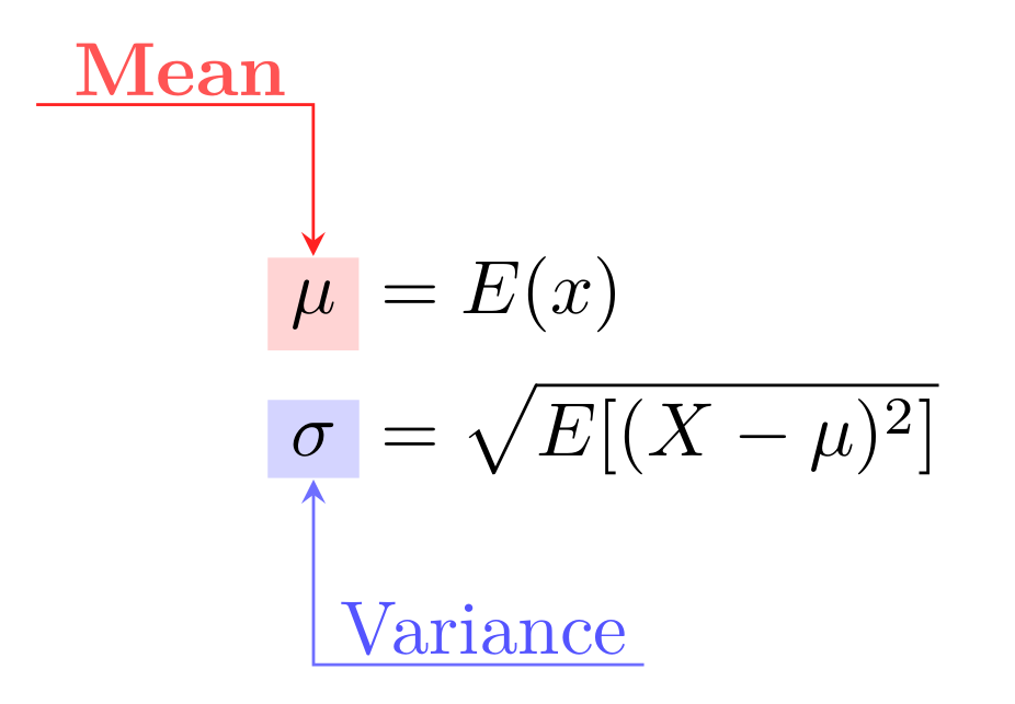
The idea is relatively straightforward: we need to think about the target of
our experiment (e.g. query latency) as a random variable X, described as a
population with a certain distribution and parameters, often median and
variance:
Now, when we conduct a benchmark and gather some results, those data points are in fact samples from this larger population. Working with benchmark results we operate with mean and variance estimations, usually simply mean and variance of the sample. Having all this in place and two sets of data – baseline results and performance after some modification – one can perform a one-sample t-test to get ρ value and say the magical phrase “the difference between two sets is significant at significance level 5%” and even provide a confidence interval. In other words, it doesn’t look like the difference we observe would have occurred due to the sampling error alone.
You don’t have to remember all of those formulas. In fact, most likely my description above would make every decent scientist feel insulted. Fortunately for us all this machinery is implemented in many libraries, e.g. SciPy. But it’s still important to understand where all this is coming from, and as you might expect there are enough caveats.
3.3 Big problem in CS
Since we work with databases, we’re a bit luckier than a scientist in the field – it’s much easier to get a lot of data. It’s always tempting to produce large set of benchmarking results and claim we can get an extraordinary high confidence level using methods described above. Yet, often it doesn’t work, because there is a big problem.
Student’s t-test is a parametric method, i.e. it has an important assumption about the data: all measurements have to be independent samples from a normal distribution [6]. The intuitive idea is that all the small random factors have to influence the final result in the same way. And this assumption holds almost all the time in natural sciences, but not always in computer science.
Data obtained from e.g. a physical experiment is often normally distributed. At the same time everything what has to do with computers usually produces a skewed distribution with quite a long tail:
Normal (Gaussian) distribution vs skewed distribution (Longtail)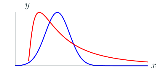
Intuitively it’s even clear why:
-
Almost every computer system is a network of queues, meaning that there is a “happy path” for a query with no congestion and waiting in a queue, and everything else will be only slower, pushing the distribution to the right and in certain cases producing significant outliers and long tail latency.
-
It’s often the case that only one factor is dominating the latency. E.g. we often speak of “IO” or “CPU” bounded workload, where the corresponding component contributing the main latency component. Thus equal contribution to the final result is compromised.
Ok, but what does it mean? The consequences are that if we use t-test we’re walking on an extremely thin ice. It might be working just fine, and in [7] authors show that parametric tests are quite robust to violation of normality assumption when we compare means. In fact, there are some examples of applying parametric tests to the real data with satisfying results, e.g. it’s used in Hunter [8] and an option for ClickHouse benchmarking tools. At the same time it might fail spectacularly if we try to compare variance (again, in [7] authors show parametric tests are more vulnerable in this case), or the underlying distribution is extremely far from normal, in the worst case a multimodal one.
There are ways to test for normality [6] if you’re not sure, but to reiterate – most of the time measurements of computer systems are taken from non-normal distributions. It’s not even that hard to reproduce this, as in the example below: PostgreSQL is running inside a cgroup, limiting how much memory the database could use, and leading to some fraction of queries being fulfilled from the memory, and the rest hitting the disk:
An example of bimodal distribution for query latency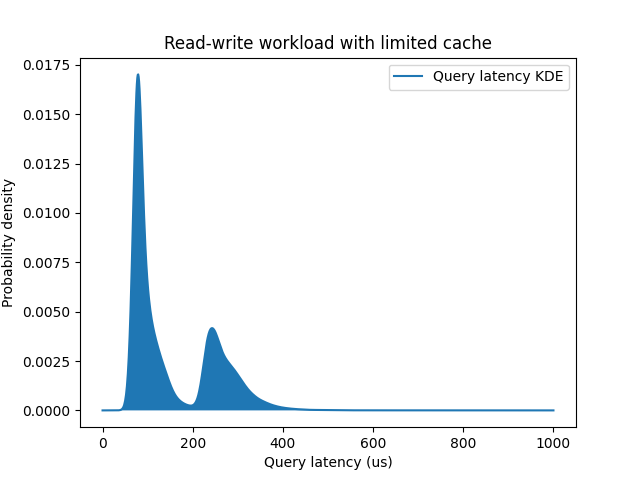
The resulting distribution is bimodal with two main contributing factors: usage of the memory cache and usage of the slower storage. The difference between two modes is about ~150 microseconds (usec), which is close to the pure IO latencies we can measure for the storage device independently:
@usecs:
[16, 32)              32 |                                          |
[32, 64)             202 |                                          |
[64, 128)         169897 |@@@@@@@@                                  |
[128, 256)        679545 |@@@@@@@@@@@@@@@@@@@@@@@@@@@@@@@@@@@@@@@@@@|
[256, 512)         20950 |@                                         |
[512, 1K)            378 |                                          |
[1K, 2K)             118 |                                          |
[2K, 4K)             133 |                                          |
[4K, 8K)             306 |                                          |
[8K, 16K)             79 |                                          |
[16K, 32K)            68 |                                          |
[32K, 64K)           104 |                                          |
[64K, 128K)           46 |                                          |
What should we do if a parametric test doesn’t work? An alternative option is to use non-parametric tests and metrics that do not make any assumptions about normality and more robust:
- Mann-Whitney U test, also implemented in SciPy.
- Median, and percentiles in general.
- IQR (inter quantile range) for outliers.
Note, that those methods are by no means a silver bullet. There are many more tests besides Mann-Whitney that have different properties, they all usually a bit more complex than parametric tests, and still do have assumptions about exchangeability.
3.4 How many runs do we need?
Now that we’ve shed some light on the topic of statistical methods for measurements comparison, there are few interesting questions to answer. How much data do we need to accumulate to draw conclusions with confidence? It’s not always possible to generate large volumes of data on demand, e.g. due to infrastructure costs or long time that it takes to perform one test round, hence it’s tempting to try minimizing amount efforts for conducting a proper performance evaluation.
The question is tricky and depends on many details, but here I would like to share an interesting article [9] that can give you at least an impression what to expect. The research topic was investigation of an unavoidable variance that comes from the hardware itself: disk IO, networking, memory access. There are so many reasons for hardware to have variable performance, it could be different temperature, timings, slowly failing hardware or even variance in manufacture.
The results are formulated as a function of coefficient of variance (CoV, the
ratio of standard deviation to the mean) and E(r, α, X) – number of
repetitions for an experiment, with set of measurements X, required to achieve
sufficiently narrow confidence interval (where r is relative difference between
CI bounds and the mean) given confidence level α. For example, for quite stable
hardware with the CoV only 0.3% one have to repeat the experiment modest 10
times, in other words E(1%, 95%, X) = 10. At the same time if we bump the
variance level to 9% (lets say, now we deal with an IO workload hitting a
disk), the number of experiments is already 240, E(1%, 95%, X) = 240. Across
all the setups the maximum number they’ve got was ~600.
3.5 Randomized testing
This brings us to another discussion – how to deal with factors we can’t really control? There is an unavoidable hardware noise, there are things we may not anticipate, there are even things out of our control by definition (like unexpected noisy neighbours if we have to use shared resources for benchmarking), all of this can affect the experiment. Fortunately, it turns out there are a couple of tricks to get reasonable results even in this case, and they have something to do with randomization.
One way would be to let those factors that we don’t control to affect both runs, the baseline and the modified one. This approach is called paired comparison design and often used in manufacturing [7]. One can think of a setup, where we compare two database configuration – a default one and a tuned one – and run both instances at the same time on the same VM. In that case even if there would be an unexpected noisy neighbour appearing, it would affect both results, and we still can compare them without problems. Of course, this leaves open the question of how to isolate those two instances and prevent from affecting each other.
Another way would be to introduce randomization in the sampling process, meaning that every measurement will randomly be taken either from the baseline or the modified run. It’s called randomized testing or randomized block testing (if we divide experiments into blocks and randomize within those blocks) and is a working horse in many industrial experiments (again [7] is a great resource on this). In context of databases it would be again similar to testing two configurations, but this time instead of running both instances on the same VM, we randomly assign every query to be sent to one or another instance. In this way even if there is something influencing the experiment introducing some correlation, the impact will be randomized away.
To be honest, I rarely see those approaches when it comes to database performance, the only example I know of is ClickHouse performance testing. But it’s ubiquitous in the industry and natural sciences, which means there is a lot to learn from.
3.6 Time average or ensemble average?
There is another question that goes in similar direction: under the same conditions, what is better from statistics perspective: to run one benchmark for longer time period, or to run many smaller benchmarks for shorter time period? Marc Callaghan asked this question some time ago, and in the linked blog post you can find many interesting takes on it. The question triggered me to do my own research, ending up writing this article, and here I want to share somewhat relevant fact I’ve discovered when reading up on statistics.
In queueing theory one can ask a similar question, but formulated differently [10]: for a stochastic process (e.g. number of jobs in a queue), is an average of a single process instance over a long time frame (a time average) equivalent to an average of many instances of the process over a shorter time frame (an ensemble average) for a data stream? It turns that for an ergodic system they are indeed equivalent:
But what is an “ergodic” system? The precise definition says [10]:
An ergodic system is one that is positive recurrent, aperiodic and irreducible.
In simple words, it’s a system where we can get from any one state to any other state, and mean time between visits to the same state is finite. The idea is that an ergodic system can sort of “forget” its own past at some point – if we start in a state 0, after some time return to the state 0, and we could think of this return as a restart of the statistical process.
Now, this all sounds rather abstract, can we somehow apply this knowledge? Can a database be considered an ergodic system? The main problem is that databases are stateful systems, and to make it close to an ergodic we need to reduce this “statefullness” (via cleaning up of inserted data, properly configured vacuuming etc.) to achieve the state when the database under load produces stable enough metrics. Thus, we end up with an obvious (but more well grounded) understanding that to make one long benchmark run equivalent to many shorter runs, we need to reach a stable state first.
4. Summary
Despite all the words I’ve spent above, we barely have scratched the surface. The topic is immense, we could talk more about how to reduce hardware noise, use machine learning to tune databases, ANOVA, factorial and split-plot designs to make benchmarking more formalized and efficient. But it’s better to stop here before things will completely get out of control.
There are few conclusions I would like to reiterate:
-
Benchmarking is exciting! It’s not about dry numbers, statistics and configuration – it’s about learning something new, about exploring the system behaviour and revealing hidden dependencies and secrets.
-
Benchmarking is an iterative process. It’s almost impossible to do a single experiment that will give definitive answer to all the questions, one have to do many iterations, improving along the way, doing cross-validation and verification of the data. Quoting [7]:
The idea that every experimental design should by itself lead to an unambiguous conclusion is of course false.
-
It’s important to keep in mind we deal with known and unknown factors. While expanding our knowledge about the system, we’re not allowed to ignore that there is still some unknown lurking around.
-
Combining “common” (statistics) and “particular” (specific domain knowledge) expertise is crucial to get the full picture of what’s going on.
-
Something that I haven’t stated clearly, but you could notice indirectly. Using statistics for benchmarking not only can help to interpret the data, but also can serve as a language to clearly explain the results and conclusions to others.
5. References
[1] Kuznetsov, N., Bonnette, S. and Riley, M.A., 2013. Nonlinear time series methods for analyzing behavioural sequences. In Complex systems in sport (pp. 111-130).
[2] Van Aken, D., Yang, D., Brillard, S., Fiorino, A., Zhang, B., Bilien, C. and Pavlo, A., 2021. An inquiry into machine learning-based automatic configuration tuning services on real-world database management systems. Proceedings of the VLDB Endowment, 14(7), pp.1241-1253.
[3] Schroeder, B., Wierman, A. and Harchol-Balter, M., 2006. Open versus closed: A cautionary tale. USENIX.
[4] Zhang, S., Heck, P. R., Meyer, M. N., Chabris, C. F., Goldstein, D. G., & Hofman, J. M. (2023). An illusion of predictability in scientific results: Even experts confuse inferential uncertainty and outcome variability. Proceedings of the National Academy of Sciences, 120(33)
[5] Student, 1908. The probable error of a mean. Biometrika, 6(1), pp.1-25.
[6] Hoefler, T. and Belli, R., 2015, November. Scientific benchmarking of parallel computing systems: twelve ways to tell the masses when reporting performance results. In Proceedings of the international conference for high performance computing, networking, storage and analysis (pp. 1-12).
[7] Box, G.E., Hunter, J.S. and Hunter, W.G., 2005. Statistics for experimenters. In Wiley series in probability and statistics. Hoboken, NJ: Wiley.
[8] Fleming, M., Kolaczkowski, P., Kumar, I., Das, S., McCarthy, S., Pattabhiraman, P. and Ingo, H., 2023, April. Hunter: Using Change Point Detection to Hunt for Performance Regressions. In Proceedings of the 2023 ACM/SPEC International Conference on Performance Engineering (pp. 199-206).
[9] Maricq, A., Duplyakin, D., Jimenez, I., Maltzahn, C., Stutsman, R. and Ricci, R., 2018. Taming performance variability. In 13th {USENIX} Symposium on Operating Systems Design and Implementation ({OSDI} 18) (pp. 409-425).
[10] Harchol-Balter, M., 2013. Performance modeling and design of computer systems: queueing theory in action. Cambridge University Press.
6. Acknowledgements
Thanks to Mark Callaghan for unintentionally triggering my research, leading to this article, Torsten Hoefler for drawing attention to common statistics issues in benchmarking and Sibin Mohan for great examples of annotated equations in latex.