Evolution of tree data structures for indexing: more exciting than it sounds
28 Nov 20200. How to read me?
I have to admit, my research blog posts are getting longer and longer. From one side I find it genuinely encouraging, because if one gets so much information just by scratching the topic, imagine what’s hidden beneath the surface! One university professor once said “what could be interesting in databases?”, and it turns out freaking a lot! On the other side it certainly poses problems for potential readers. To overcome them I would suggest an interesting approach: print this blog post out, or open it on your tablet/e-reader, where you can make notes with a pencil or markers. Now while reading it try to spot ideas particularly exciting for you and mark them. Along the way there would be definitely some obscure parts or questions, write them on the sides as well. You can experiment with the diagrams, changing or extending them, or just drawing funny faces. But do not read everything at once, have no fear of putting it aside for a while, and read in chunks that are convenient for you. Some parts could be skipped as the text is build out of relatively independent topics. The table of contents can help and guide you. Having said that we’re ready to embark on the journey.
- Introduction
- RUM conjecture
- B-tree basics
- Beyond the hard leavers of basics
- Why is it not enough?
- Trie
- Learned indexes
- Is that all?
- References
1. Introduction
Whenever we speak about indexes, especially in PostgreSQL context, there is a lot to talk about: B-tree, Hash, GiST, SP-GiST, GIN, BRIN, RUM. But what if I tell you that even the first item in this list alone hiding astonishing number of interesting details and years of research? In this blog post I’ll try to prove this statement, and we will be concerned mostly with B-tree as a data structure.

Let’s start systematically and take a look at the definition first:
B-tree is a self-balancing tree data structure that maintains sorted data and allows searches, sequential access, insertions, and deletions in logarithmic time.
What is your first association with the concept of B-tree? Mine is “old and well researched, or in other words boring”. And indeed apparently it was first introduced in 1970! Not only that, already in 1979 they were ubiquitous. Does it mean there is nothing exciting left any more? Once upon a time I came across a remarkable read called Modern B-Tree techniques which inspired me to dig deeper into the topic and read bunch of shiny new whitepapers. Afterwards totally by chance I’ve stumbled upon a book “Database Internals: A Deep Dive into How Distributed Data Systems Work”, which contains great sections on B-tree design. Both works were the triggers to write this blog post. What was I saying about nothing exciting left? At the end I couldn’t be more wrong.
It turns out that there are multitude of interesting ideas and techniques around B-Trees. They’re all coming from the desire to satisfy different (often incompatible) needs, as well as adapt to emerging hardware. To demonstrate how many of those exist, lets play a game. Below you can find a table of names I’ve found in various science papers, together with a couple of silly names I’ve come up myself. Can you find out the fake ones?
| B-tree | B+-tree | Blink-tree | DPTree |
| wB+-tree | NV Tree | FPTree | FASTFAIR |
| HiKV | Masstree | Skip List | ART |
| WORT | CDDS Tree | Bw Tree | HOT |
| KISS Tree | VAST Tree | FAST | HV Tree |
| UB Tree | LHAM | MDAM | Hybrid B+ Tree |
Any ideas? Well, I have a confession to make – all of them are real, I just don’t have enough imagination to come up with such names. Having this in mind hopefully you understand that if we want to make a survey, the first step would be to establish some classification. Not only this will help us to structure the material, but also will explain why on earth anyone would need to invent so many variations of what we though was so simple!
2. RUM conjecture
To classify different index access methods we need to think about the following ambitious question – is there anything common between almost any index access method? The authors of RUM conjecture provide an interesting insight about this topic:
The fundamental challenges that every researcher, systems architect, or designer faces when designing a new access method are how to minimize, i) read times, ii) update cost , and iii) memory (or storage) overhead.
In this paper, we conjecture that when optimizing the read-update-memory overheads, optimizing in any two areas negatively impacts the third
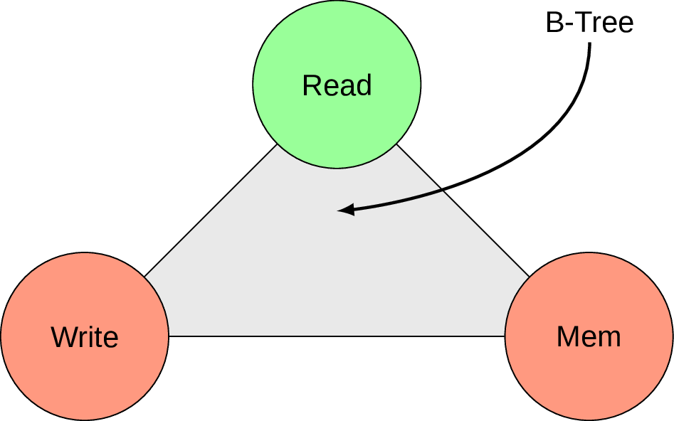
This essentially states that if an index access method could be specified as a point inside “Read”, “Update” (on the Fig. 1 it’s called “Write” for convenience of drawing), “Memory” space we can observe an interesting invariant. Every time we modify one index access method to have less overhead for reading or memory footprint (i.e. shift the corresponding point closer to “Read”/”Memory” corners), we inevitably loose on the updating workload (i.e. getting further away from “Write” corner).
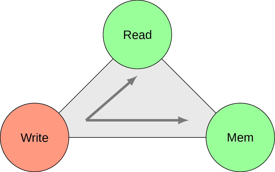
In fact as a non-scientist I would even speculate that there should be another dimension called “Complexity”, but the idea is still clear. I will try to show this invariant at work via examples in this blog post, but it already gives us some ground under the feet and opportunity to visually represent different versions of B-tree by moving point on the triangle back and forth. But first let’s recall the basics.
3. B-tree basics
So what is B-tree? Well, it’s a tree data structure: a root node, some number of branch nodes (marked grey) and a bunch of leaf nodes (marked green):
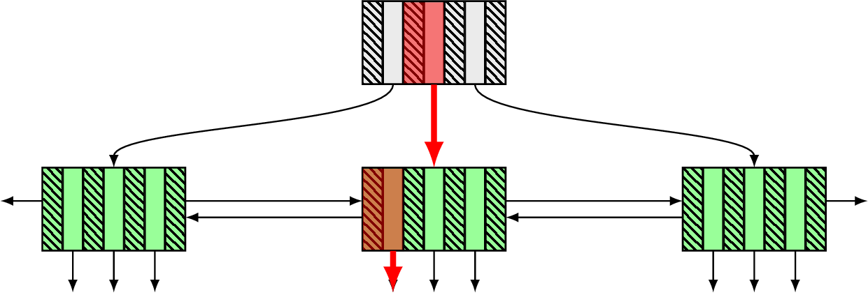
Every node of this tree is usually a page of some certain size and contains keys (shaded slices of a node) and pointers to other nodes (empty slices with arrows). Keys on page are kept in sorted order to facilitate fast search within a page.
The original B-tree design assumed to have user data in all nodes, branch and leaf. But nowadays the standard approach is a variation called B+-tree, where user data is present only in leaf nodes and branch nodes contains separator keys (pivot tuples in PostgreSQL terminology). In this way separation between branch and leave nodes become more strict, allowing better flexibility for choosing format of former and making deletion operations can affect only latter. In fact the original B-tree design is barely worth mentioning these days and I’m doing this just to be precise. Since B+-tree is sort of default design, we’ll use B-tree and B+-tree interchangeably in this text from now on. An interesting thing to mention here is that the only requirements for separator keys is to guide search algorithm to a correct leaf node. As long as they fulfil this condition they can contain anything, no other requirements exist.
Strictly speaking, only child pointers are truly necessary in this design, but quite often databases also maintain additional neighbour pointers, e.g. what you can see on the Fig. 2 between the leaf nodes. It could be helpful for some operations like index scan, but need to be taken into account for node split/merge operations. PostgreSQL uses Lehman-Yao version, called Blink-tree, with links to both left and right sibling nodes (the left link one is actually not presented in the original Blink-tree design, and it makes backward scan somewhat interesting), and there are even implementations like WiredTiger with parent pointers.
Having all this in place one can perform a search query by following the path marked red on the Fig. 2, first hitting the root, finding a proper separator key, following a downlink and landing on a correct page where we deploy binary search to find the resulting key.
Until now, we were talking only about static parts of B-tree design, but of course there is more to it. For example there is one dynamic aspect of much importance (quite often it even scares developers like a nightmare), namely page splits. What do we need to do when there is a new value to insert, but the target page does not have enough space like on the following diagram?
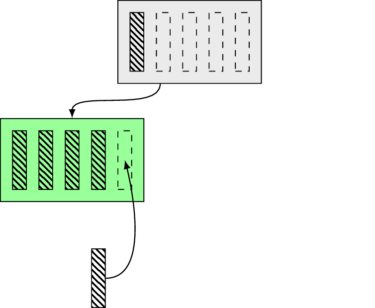
What happens here is we’re trying to insert the new value (shaded box) into the page with not enough space for it. To maintain the three balanced we need to allocate another leaf page, distribute keys between old and new leaf, promote a new separator key into the parent page and update all required links (left/right siblings if present):
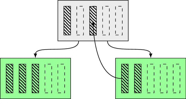
Curiously enough the new separator key could be chosen freely, it could be any value as long as it separates both pages. We can see what does it change in the optimization section.
Locking is obviously an important part of a page split. No one wants to end up with concurrency issues when pages get updated while in the middle of a split, so a page to be split is write-locked as well as e.g. right sibling to update left-link if present.
As you can see, page splits are introducing performance overhead. We need to bring in a new page, move elements around and everything should be consistent and correctly locked. And already at this pretty much basic point we already can see some interesting trade-offs. For example B*-tree modification tries to rebalance data between neighbouring nodes to postpone page split as long as possible. In terms of trade-offs it looks like a balance between complexity and insert overhead.
I didn’t tell you everything about Blink-tree and it’s going to be our next topic example in this section. Not only Lehman-Yao version adds a link to the neighbour, it also introduces a “high key” to each page, which is an upper bound on the keys that are allowed on page. While obviously introducing a bit memory overhead those two changes make it possible to detect a concurrent page split by checking the page high key, which allows the tree to be searched without holding any read locks (except to keep a single page from being modified while reading it) [6]. We can think of it as a balance between memory footprint and insert overhead.
We’ve spent so much time talking about page splits and their importance. For the sake of symmetry one can expect the same from page merges, but surprisingly it’s usually not the case. There is even the paper that states:
By adding periodic rebuilding of the tree, we obtain a data structure that is theoreticaly superior to standard B-trees in many ways. Our results suggest that rebalancing on deletion no only unnecessary but may be harmful.
But of course vacuum in PostgreSQL can still reclaim empty pages (see “Page Deletion” in [6]).
Now just to get taste of a real B-tree let’s generate an index in PostgreSQL and visualize it. The easiest way would be probably to create a small data set with pgbench and then plot the resulting graph of B-tree nodes and connections using a script from pg_query_internals, you can see the result on Fig. 4:

Are you confused, what is this bumpy line? Well, it’s my attempt to fit the visualization into the screen, because in reality B-trees are extremely wide. Now let’s play a bit and modify the visualization script to show every node as a small dot and use “neato” layout for graphviz:
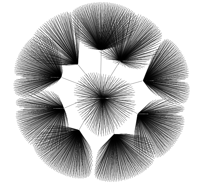
Fig 5. demonstrates nicely another observation about B-trees, they’re indeed extremely wide, short and even sort of bushy. And the very same picture can also help us to understand another important aspect of B-tree that makes it indeed ubiquitous in database systems. The reason is that with B-tree one can address many kinds of workloads with reasonable efficiency, it’s not designed with only one target in mind. How is that possible? It’s thoroughly explained in “Modern B-tree techniques”, particularly in “B-tree versus Hash Indexes” section, so I’ll just formulate the summary.
For one, B-tree can effectively exploit memory hierarchy, because as you can see it’s extremely wide, and if an index is “warm” it means most likely all branches nodes will be present in the buffer pool or could be fetched into the buffer pool while preparing the query. For leaf pages an efficient eviction policy could be deployed as well to address non-uniform workload. In general space management in B-tree is rather straightforward and an index can grow or shrink smoothly, whereas graceful grow or shrinking e.g. hash indexes is not fully solved yet.
Another property of B-tree that helps to address different workloads is its ability to support different form of queries (search with a prefix of the index key, or index skip scan) using only one index.
Last but not least is B-tree flexibility in terms of optimizations. One could compose different optimizations at different levels to be able to address some particular type of workloads mostly without negatively affecting performance in other cases.
Having said all that we can also pinpoint where in the RUM space we can place B-tree. Since it’s pretty good in read workload, but could be better with memory footprint and insert workload, we can put it somewhere here:
4. Beyond the hard leaves of basics
As we already mentioned, one of the reasons why B-trees are so universal in the databases world is their flexibility and extensibility. On can apply variety of different local optimizations which could be nicely composed without sacrificing on something else. Let’s take a loot at some of them.
4.1 Key normalization
Probably the simplest we can do is key normalization, which is apparently a quite old technique [3]. The idea is pretty simple, if there is an index record with several keys for every column we transform them into a binary string like on Fig. 7:
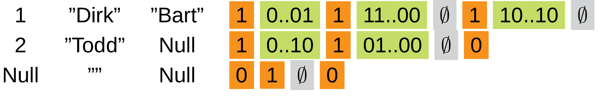
This allows to use simple binary comparison to sort the records during index creation or when guiding a search to the correct record. Such an encoded value need to take care about nulls and collations and can even include sort direction. But as always there are pros and cons and in this particular case the trick is that generally speaking it is impossible to reclaim the original data. In certain situations it can even happen that two different values produce the same normalized key (e.g. for languages with lower/upper case sorted case-insensitive). This means that we either:
-
need to keep both original data and normalized key or somehow else make sure precise recovery is possible.
-
use key normalization only for branch nodes.
By itself this modification looks pretty innocent, but in fact it enables us to implement more optimizations on top of it.
4.2 Prefix truncation
One of such optimizations, which could be much easier implemented with the help of normalized keys is prefix truncation. And you will be surprised how straightforward it is. Imagine we have the following keys on one page:

Note that the value we store start with the same prefix, which is sort of data duplication. If we’re going to do a bit of bookkeeping, it’s possible to store this prefix only once and truncate it from all the keys.

As you can imagine this optimization is about trade-off between consuming less space on leave pages, but doing more job at run-time. To reduce code complexity and run-time overhead, usually prefix truncation is done over the whole possible key range based on fence keys (those are copies of separator keys posted to the parent during split), although more fine-grained approach can give better compression ratio (and more headache for insert operation).
One example of databases using this approach is Berkeley DB.
4.3 Dynamic prefix truncation
Even if prefix truncation is not implemented directly and B-tree pages format is not changed, dynamic prefix truncation could be used to reduce comparison costs based on the knowledge about shared prefix and fence keys. Following the diagram on Fig. 9, if we want to add a new key (an outstanding item) and fence keys on a page have common prefix (marked as red parts), it means all the keys have it and could be omitted from comparison (leaving us with only blue part to deal with):
You may also know this approach under common prefix skipping name in the context of sorting algorithms. Unfortunately terminology inconsistencies happen relatively often as you can notice throughout the whole blog post (another interesting example is B*-tree, which called “most misused term in B-tree literature” in Ubiquitous B-tree).
4.4 Suffix truncation
Despite the similar name, suffix truncation is a bit different beast. This trick could be applied to separator keys on branch pages and the easiest way to explain it is to show the diagram. Let’s say we have a page to split:

In case if this page would be split right in the middle, we end up with the key “Miller Mary”, and to fully distinguish splitted parts the minimal separation key should be “Miller M”. But as I’ve mentioned above we can actually choose any available separation key as long as it separates both pages, so why not take something shorter like in the following example?

That is pretty much the whole idea, to pick up a split point in a such way that the resulting separation key will be minimal.
Worth mentioning that starting from version 12 PostgreSQL does whole-colum suffix truncation without actually implementing key normalization. There is even a good overview of all these techniques in the corresponding wiki page.
4.5 Indirection vector
Normally we have to deal with values of variable length, and the regular approach to handle them is to have an indirection vector on every page with pointers to actual values. In PostgreSQL terminology those pointers are called line pointers. Every time when we have a key to compare, we first follow a pointer and fetch the value it points to. But what if we extend this design a bit and equip every such pointer with some useful information, for example a first few bytes of the normalized key we’re going to find after following the pointer, as with the diagram on Fig. 12 (e.g. first characters a,b,c,d)?
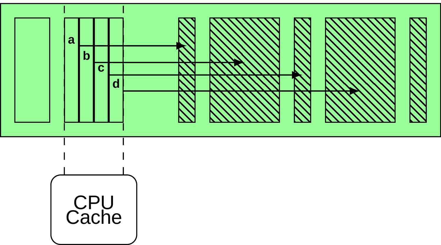
Such a small change allow us to figure out if the value we’re looking for could be not found following this pointer since the first few bytes are already different. This makes the design more CPU cache friendly, as the indirection vector is usually small enough to fit into the cache. For more details take a look at [9].
Another interesting approach I find somehow similar is overflow pages, when only a fixed number of payload bytes is actually stored in the page directly and the rest goes to the overflow page. Few examples are MySQL InnoDB and SQLite.
4.6 SB-tree
Page splits are a big deal in B-tree design, and obviously interesting variations could be found in the wild about how to deal with them. SB-tree is one such example, where to improve page split efficiency disk space is allocated in large contiguous extents of many pages. This leaves free pages in each extent and whenever a node needs to be split, another node is “allocated” within the same extent from already preallocated space, like in the following diagram on Fig. 13:
Of course, it means that an extent itself could reach the point when there is no more free space and it needs to be split following the same ideas as normal page split. You maybe surprised what SB-tree is doing here, in basics section, since it’s not a standard approach. Yes, it’s not basic, but I’ve decided to mention it here anyway mostly due to its almost intuitive idea.
5. Why is it not enough?
Indeed, everything looks great, why do we need to come up with some other designs? Well, as you can remember on the RUM space we put B-tree closer to the “Read” corner and not without the reason. There are several common downsides of B-tree design:
-
It’s not particularly CPU cache friendly due to pointer-chase, since to perform an operation we need to follow many pointers.
-
Memory footprint and insert performance are located on different sides of balance, we can improve inserts by preallocating pages and keep track of free space on the page which requires more memory. The same is valid for data compression.
-
B-tree requires lock coupling on page level to synchronize an access, which doesn’t scale that well on many-core CPUs or in-memory systems (see [10], [11]).
-
Bulk inserts is also not particularly efficient out of the box, and in general index maintenance could be pretty tricky (my favorite description of this part is paper “Waves of Misery After Index Creation”).
At the same time there are some alternative data structures that provide similar functionality but different set of trade-offs. All this makes the topic pretty dynamic and full of interesting ideas. I’ll try to describe some of those designs I find interesting in the following sections. Keep your eyes opened, you will probably notice many common patterns.
5.1 Partitioned B-tree
If SB-tree could be called intuitive, partitioned B-tree idea sounds rather confusing at first. Essentially the suggestion is to maintain partitions within a single B-tree via adding an artificial leading key field (see [14]). Those partitions are nothing but temporary, and after some time will be merged together in background so that in the normal state there is only one partition. Why on earth would we add artificial data to an index, which is clearly an overhead? The original paper suggests that this design could be beneficial if we need to assemble an index from smaller chunks. For example if we want to build a new index from number of merge sort runs. Normally what happens is that intermediate sort runs are kept separately, and in case if we maintain partitions within a B-tree it’s possible to store these intermediate runs as partitions:
This makes a B-tree available for queries much earlier effectively reducing index creation time. Of course at the beginning it will not deliver the same performance due to partitions overhead, but as soon as partitions will be merged this overhead disappears. This whole approach not only makes the index available earlier, but also makes resources consumption more predictable.
After I originally discovered this approach, I’ve got an impression that unfortunately it never went further and ended up being just a curiosity. But then I’ve found more recent paper with somewhat similar ideas [15]. The main idea here is to have one partition to accumulate all inserts, updates or deletes and all the others are immutable:
This special partition is stored in a separate area called PBT-Buffer (Partitioned B-Tree) which is supposed to be small and fast. As soon as PBT-Buffer gets full it selects a victim partition and writes it out sequentially to secondary storage. Once a partition is evicted a new one is created. Another important optimization is that every partition has a corresponding bloom filter, which allows excluding partitions that do not have required key.
One can think of partitioned B-tree as few B-trees combined to produce a more complicated structure. For me the idea of using B-tree as a part of something bigger was quite a revelation. It turns out that similar ideas about incorporating multiple smaller data structures, immutable partitions and bloom filter found their representation in other researches as well. Obviously you can also note how close this design comes to LSM, in fact some LSM implementations also use a B-tree per sorted run.
5.2 Hybrid indexes
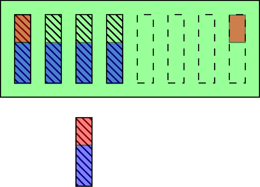
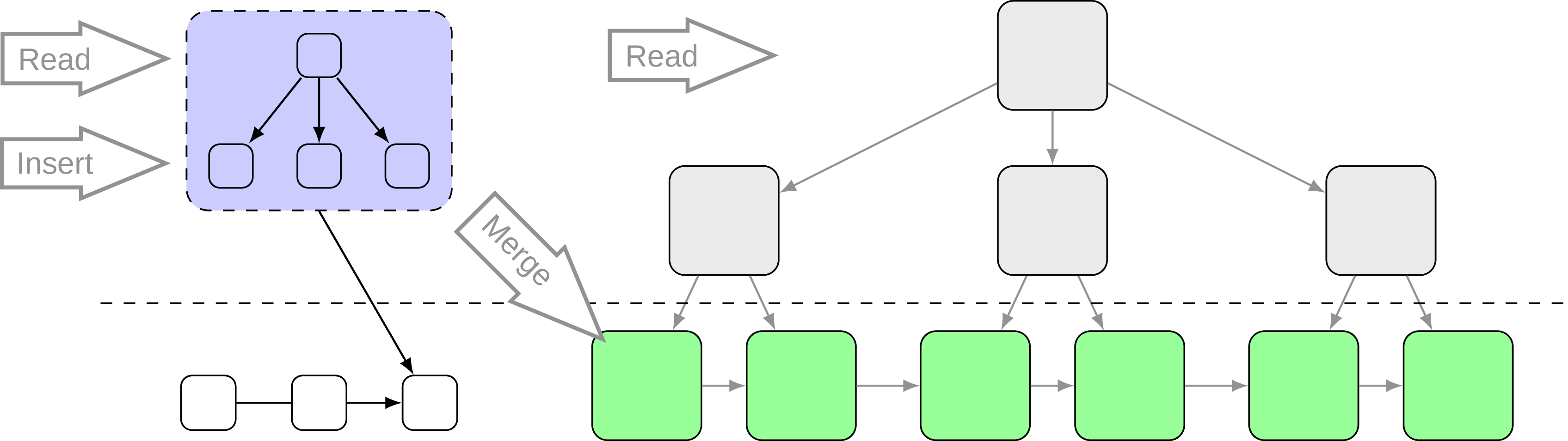
What would you do to optimize B-tree memory footprint? Normally I would answer “nothing, it’s good as it is”, but in the context of in-memory databases we need to think twice. One of interesting suggestions could be derived directly from understanding of insert performance/memory footprint trade-off. So, we want to reduce memory consumption, but still do reasonably good on insert. Why not use for that two different things at once? The authors of hybrid index suggests a dual-stage architecture with a dynamic “hot” part to absorb writes and read-only “cold” part to actually store compacted data. Obviously dynamic part is being merged from time to time into the read-only part. In fact there could be pretty much anything in place of “hot” part, but the simplest way to do it is to use B-tree as well:
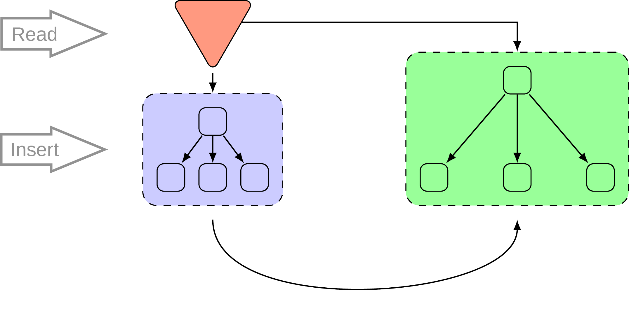
Due to read-only nature of the “cold” or “static” part the data in there could be pretty aggressively compacted and compressed data structures could be used to reduce memory footprint and fragmentation. The original whitepaper [16] is pretty entertaining and contains more rigorous explanations, I’m just abusing my status as non-scientist here to do a bit of hand-waving.
5.3 Bw-Tree
Fine, we can do something about memory footprint, what about multi-core scalability? It’s another hot topic, often mentioned in the context of main memory databases, and one interesting approach to tackle the question is Bw-tree and its latch-free nature.
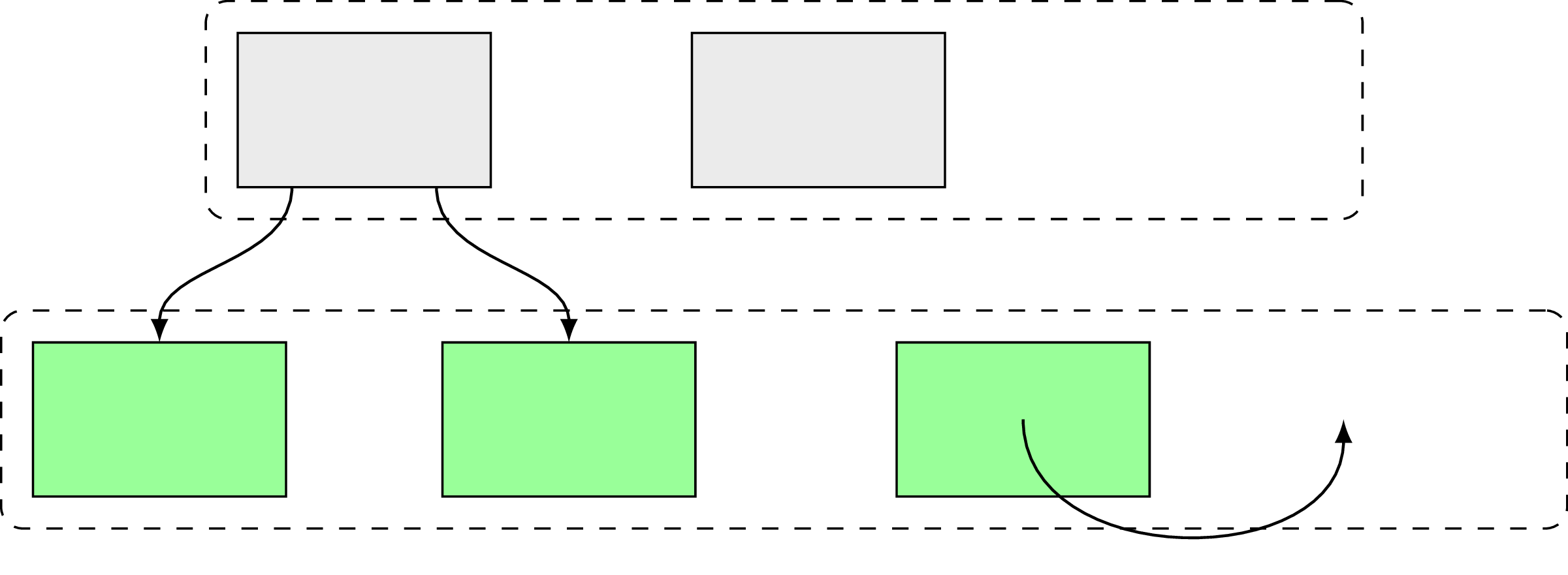
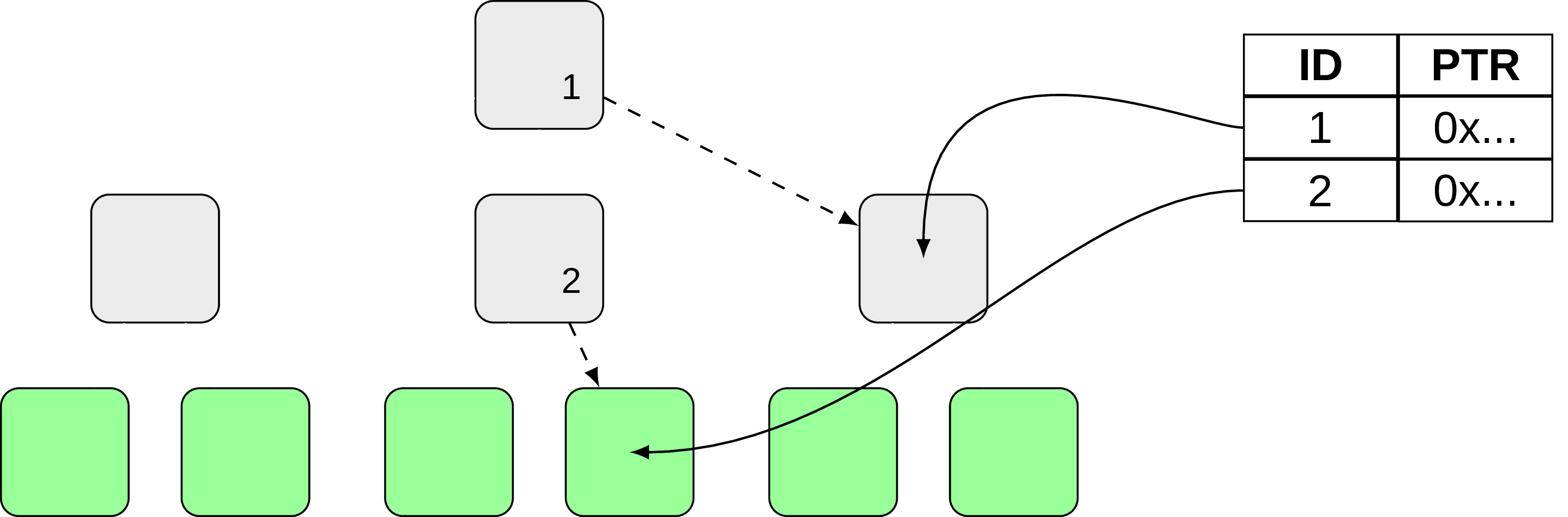
Let’s break it down into small points. First thing to notice is that Bw-tree avoids using physical pointers to pages, using logical pointers and a mapping table (which maps a logical pointer to a particular page) as an extra level of indirection:
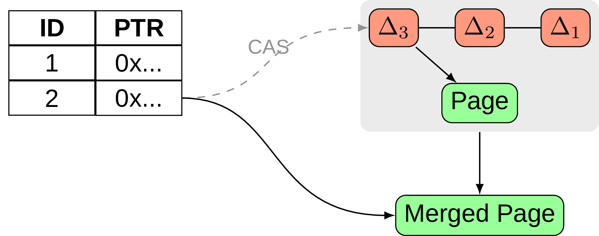
This change, while not being particularly unique by itself, enables us to implement another important part, namely delta updating. And the idea is again vaguely reminds me something about immutable pages from previous sections. So instead of doing any direct modifications on the page, let’s add a delta record describing the change, then perform an atomic CAS (compare-and-swap) to change the corresponding logical pointer so that it will point not to the original page, but to a delta record (the authors in [17] call this process “installing a new page”). The next change will introduce another delta record, which are forming a delta chain and at some point will be consolidated into a new merged page, like on Fig. 18:
The thing is it works pretty well for data modifications, but structure modifications are getting more complicated and require a split delta record, merge delta record, node removal delta record. Overall Bw-Tree performance is tricky, benchmarks shows that even with some optimizations it could be outperformed by other in-memory data structures.
Few examples of databases using this type of index are in-memory database Hekaton, embeddable Sled (although the latter one moved away from it with time), Cosmos DB and fresh NoisePage.
5.4 DPTree
In previous sections we were discussing a lot of intriguing ideas, which explore different possibilities in the index access method design to achieve something new. It’s already a vast field, and then comes a tectonic plate shift and opens even more to discover. One example of such changes is non-volatile memory and DPTree as a question how could we exploit it. One of the main issues with using persistent memory for index structures is write-back nature of CPU cache which poses questions about index consistency and logging. To prevent that we need to use fencing (e.g. clwb + mfence instructions for x86), which is somewhat similar to fsync and write-back cache. But a lot of fencing is introduces an obvious overhead, so how to find a balance here? The authors of DPTree propose dual-stage index architecture (hm…where did we see this already?):
Here we have the buffer tree, which resides in DRAM and absorbs incoming writes. This part is backed up by a redo log stored in persistent memory. When the buffer tree reaches certain size threshold, it’s being merged in-place (thanks to non-volatile memory byte addressability feature) into a base tree, which represents the main data and lives in persistent memory as well. After such merge all changes are flushed with a little fencing overhead. One interesting thing about the base tree is that only its leaves are kept in persistent memory, and all the branch nodes are stored just like that in DRAM. On crash internal nodes and required meta information is rebuild cooperatively with some running query.
There is much more to it than I’ve just described, i.e. efficient concurrent implementation of DPTree and other alternatives. I can only direct an interested reader to the whitepaper for more details.
It’s remarkable that sometimes research in this area turns into a reverse engineering, like in case of LB+-tree, where the authors were guided by discoveries and assumptions about 3DXPoint (on which Intel Optane persistent memory is based), e.g. that number of modified words in a cache line doesn’t matter for performance.
6. Trie
Now let’s try to expand our exploration area a bit more. What is it about those alternative data structures I’ve mentioned above? Are they even a thing?
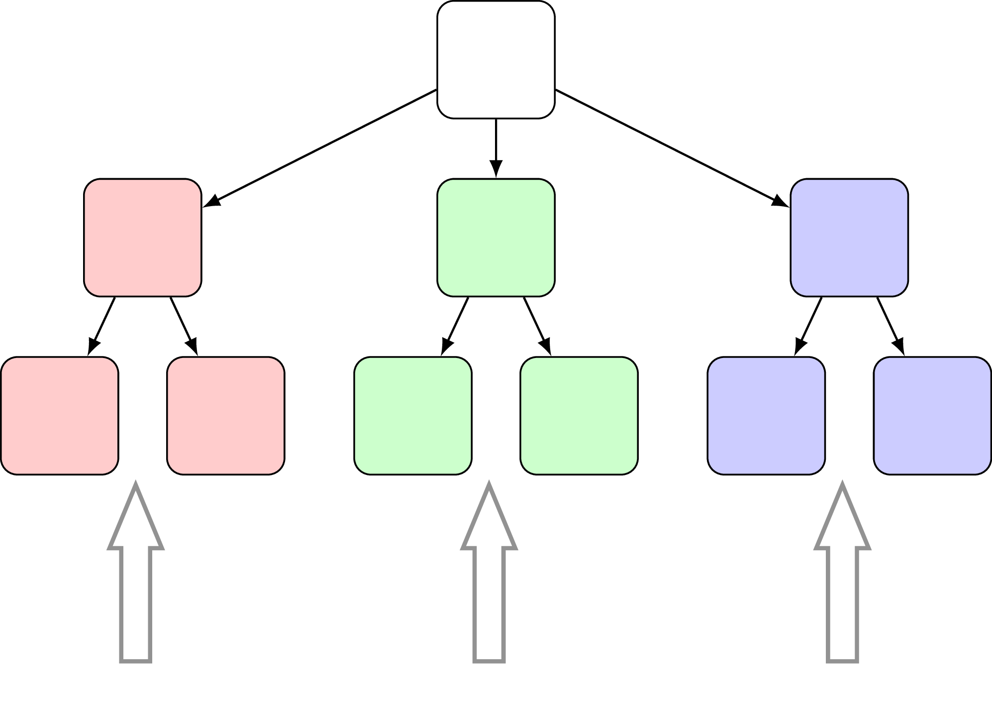
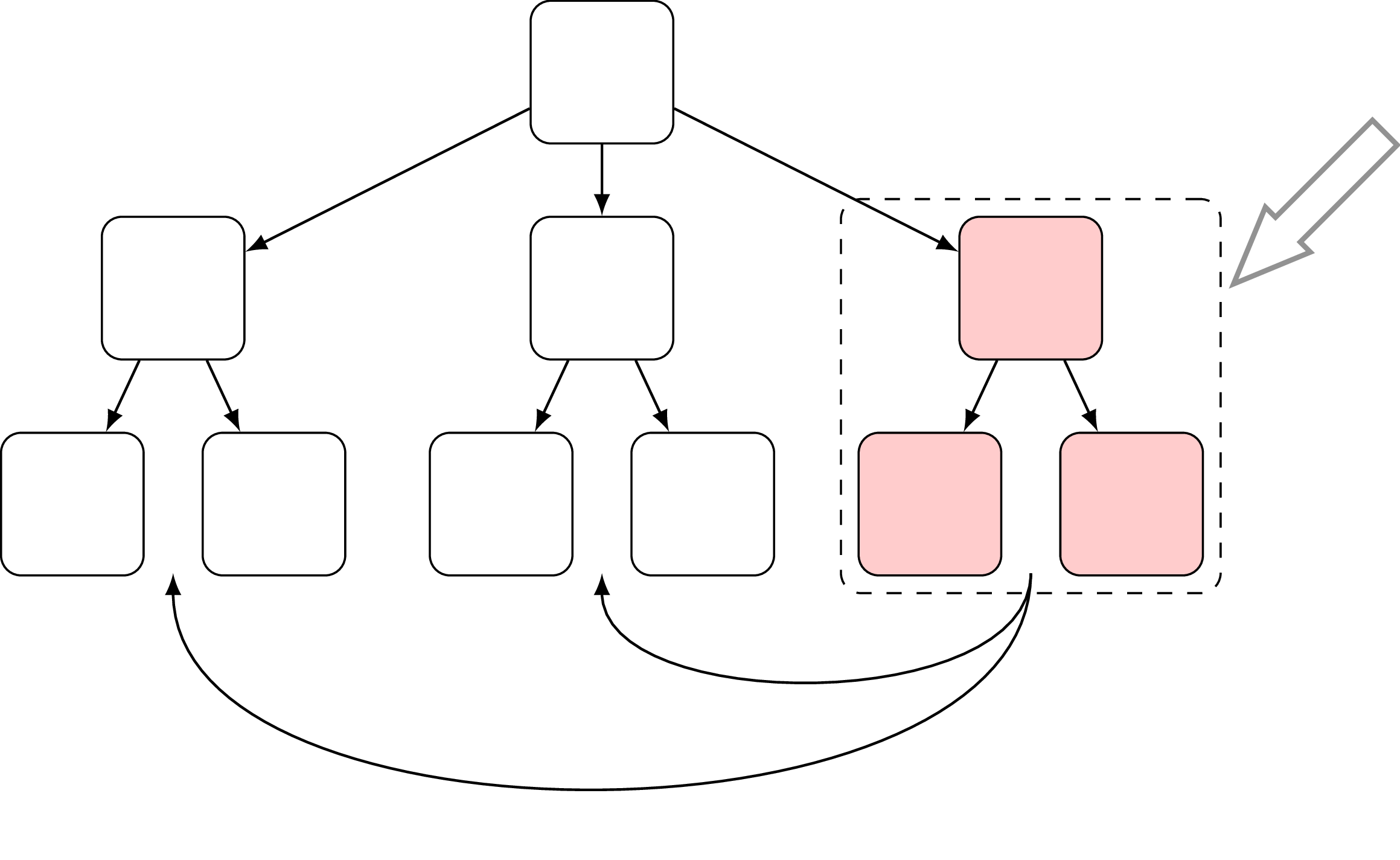
It turns out yes, and the data structure with confusing pronunciation Trie (/ˈtriː/) is one of them. Do not be surprised if you know it as a radix tree, prefix tree or even digital search tree – it’s still the same. Generally speaking trie is a search tree where the value of the key is distributed across the structure, and all the descendants of a node have a common prefix of the string associated with that node. In a way it’s similar to a thumb-index found in many alphabetically ordered dictionary books, when the first character of a word could be used to jump right away to all words starting with that character. Take a look at the example below, and try to follow one path from top to bottom assembling values on the way:
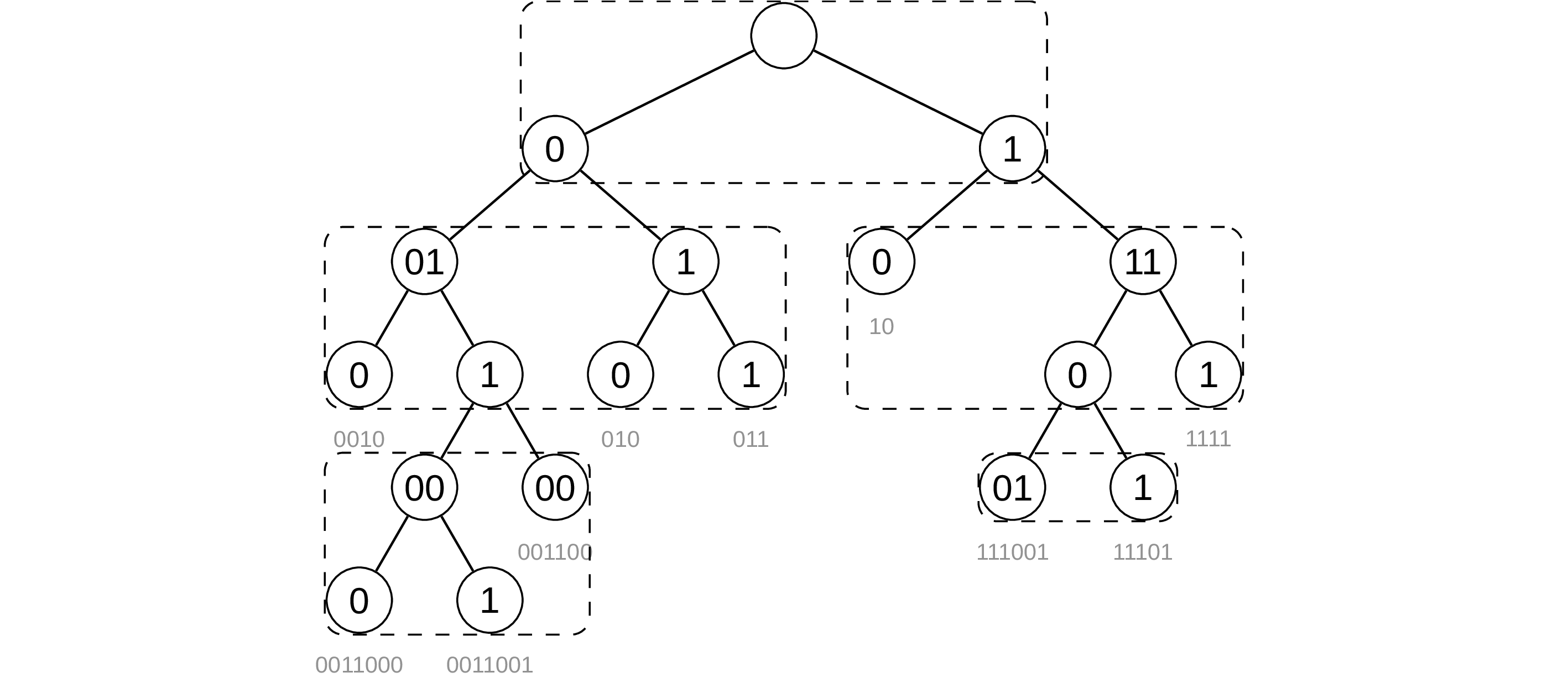
The main difference from B-tree here is that the tree heigh depends not on the number of elements in the tree, but rather on the length of the keys (and its value distribution). I already see you, confused like Ryan Reynolds, asking why do we even need to bother with all that? The idea is that a well-designed trie could be more memory efficient than B-tree and utilize SIMD instructions to perform multiple comparisons at once [19], [20]. Binary tries are too simple and of course do not provide good performance due to large tree heigh, it’s correct. But there are many techniques to reduce the heigh by creating a “compound” nodes, which are a result of combining several binary nodes together (dashed nodes in the diagram on Fig. 20). But the question of how exactly to create such nodes is not that easy, especially in the presence sparsely of distributed keys. For example Adaptive Radix Tree uses one most suitable of four node types for every group and adapt better to distribution of keys. It’s not always enough, so Height Optimized Trie goes even further and suggest adapting every compound node depending on the data distribution to limit tree heigh by some predefined value (something like in the following diagram, where each colour representing a node):
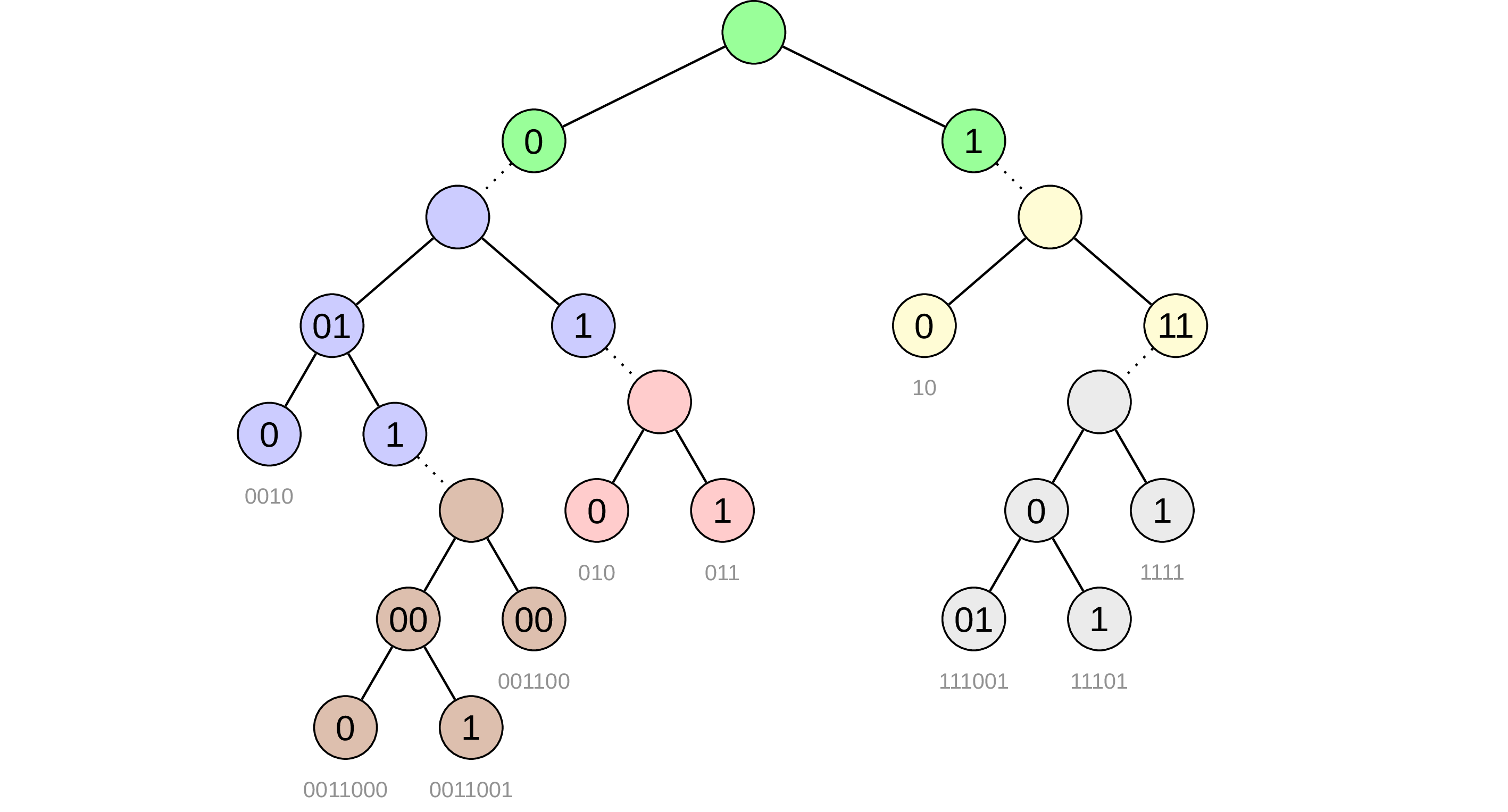
In return for all these complications we get possibility to use node layout that allow us searching multiple keys in parallel via SIMD instructions.
Another interesting example in this series is Masstree, which is a trie where every node is a B-tree, and each node handles only a fixed-length slice of a variable-length key. Such design allows supporting efficiently many key distributions, including variable-length binary keys where many keys might have long common prefixes.
Few examples of using these ideas are Silo in-memory database, ClickHouse with another modification called B-trie being used, main-memory-based relational DBMS HyPer, ForestDB key-value storage engine based on HB+-Trie, and there are discussion about using trie for Cassandra.
7. Learned indexes
To attract more readers I’ve decided to add one section about machine learning…

Never mind the joke, it turns out there are a lot of fascinating ideas arise when one applies machine learning methods to indexing. But let’s start from the beginning.
Already “Modern B-tree techniques” mentions interpolation search, the key idea of which is to estimate the position of the key we’re looking for on the page instead of doing binary search. Of course this requires some knowledge about the data distribution, at the very least we need to know if e.g. linear estimation is going to be good enough.
The authors of [21] say more, what if we replace the whole index structure with a neural network that will learn the data distribution to “predict” position of any entry in a database? In this case we get something similar to B-tree, except searching through a tree we find a page where the key is located and predicting the key location we get its position with some predefined error range. It’s possible to formalize this if we notice that “position” we’re talking about is proportional to a cumulative distribution function (CDF) since the dataset is ordered.
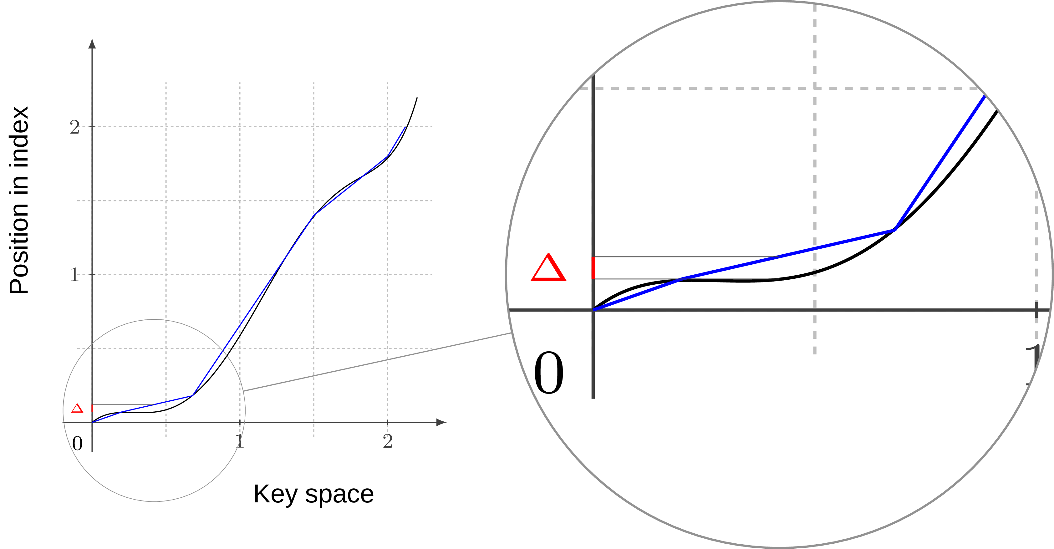
At the moment there are few different suggestions for approximating CDF, one can go with a neural network (like here [21]) or do polynomial interpolation using piece-wise linear functions (like here [23]) and more fancy stuff with Chebyshev/Bernstein Polynomial (like here [22]). For example on the plot below (Fig. 22) you can see the idea behind the interpolation, where CDF function between key space and position in index is being roughly approximated by linear segments, which of course introduces and error (marked as red delta):
But the trade-offs in both cases are in fact pretty similar:
-
On one side this gives a new flexibility dimention, now we can tune an index to consume less space but be less efficient by making it more coarse and working with bigger error intervals.
-
On the other side the model has to learn new incoming data, and it’s hard. One could train a neural network incrementally, or amortize inserts, but it’s not exactly a solved problem.
Overall we can probably put learned indexes even more far away from the insert corner of RUM space.
8. Is that all?

We have discussed so many topics, only the strongest have made to this point! But there is always more out there, the story is never fully completed. Off the top of my head we haven’t (and we’re not going to) talked about:
-
Buffered (Lazy) B-Tree
-
Cache conscious B-Tree
-
UB-Tree
-
Skip List
-
LSM stuff
-
And I’m sure much more.
In fact, I would be very interested to know if you can suggest more, let me know in the commentaries.
Now you may ask what for you may need all this information, isn’t it too academical?
Yes, it is too academical in a way, but you should not be afraid of it. No one is going to ask you about Bw-Tree on an interview (hopefully), but throughout the blog post I have tried to show that pretty theoretical stuff could be very entertaining and even inspiring at times. And theory tend to become a practice one day after all.
One more thing I want to do is to express my appreciation to all those authors I’ve mentioned in the blog post, which is nothing more than just a survey of interesting ideas they come up with. I’ve tried to carefully collect all the references below in no particular order, so you can check them out directly (I’ve probably messed up the format of the references to make them more compact, do not get mad if you’re a professional scientist).
Acknowlegements
Thanks a lot to Mark Callaghan (@MarkCallaghanDB), Peter Geoghegan ( @petervgeoghegan) and Andy Pavlo (@andy_pavlo) for review and commentaries!
References
[1] Bayer R., McCreight E. (1970). Organization and maintenance of large ordered indices. Proceedings of the 1970 ACM SIGFIDET Workshop on Data Description, Access and Control. doi:10.1145/1734663.1734671.
[2] Comer D. (1979). The Ubiquitous B-Tree. Computing Surveys, 11 (2). doi:10.1145/356770.356776.
[3] Graefe G. (2011). Modern B-Tree Techniques. Foundations and Trends in Databases. doi:10.1561/1900000028.
[4] Manos A, Stratos I. (2016). Designing Access Methods: The RUM Conjecture. EDBT. doi:10.1145/2882903.2912569.
[5] Lehman P., Yao S. (1981). Efficient Locking for Concurrent Operations on B-Trees. ACM Transactions on Database Systems. doi:10.1145/319628.319663
[6] PostgreSQL nbtree: src/backend/access/nbtree/README
[7] Sen S., Tarjan R. E. (2009). Deletion without rebalancing in multiway search trees ACM Transactions on Database Systems, doi:10.1007/978-3-642-10631-6_84
[8] PostgreSQL Wiki: [Key Normalization][https://wiki.postgresql.org/wiki/Key_normalization]
[9] Graefe G., Larson P. (2001). B-tree indexes and CPU caches, International Conference on Data Engineering, doi:10.1109/ICDE.2001.914847
[10] Kissinger T., Schlegel B., Habich D., Lehner W. (2012) KISS-Tree: smart latch-free in-memory indexing on modern architectures. In Proceedings of the Eighth International Workshop on Data Management on New Hardware. doi:10.1145/2236584.2236587
[11] Leis V., Scheibner F, Kemper A., Neumann T. (2016). The ART of practical synchronization. In Proceedings of the 12th International Workshop on Data Management on New Hardware. doi:10.1145/2933349.2933352
[12] Glombiewski N., Seeger B., Graefe G. (2019). Waves of Misery After Index Creation. BTW 2019. Gesellschaft für Informatik. doi:10.18420/btw2019-06
[13] O’Neil P. E. (1992). The SB-tree: An index-sequential structure for high performance sequential access. Acta Informatica. doi:10.1007/BF01185680
[14] Graefe G. (2003). Sorting and indexing with partitioned B-Trees, Classless Inter Domain Routing, 2003
[15] Riegger C., Vincon T., Petrov I. (2017). Write-optimized indexing with partitioned b-trees. doi:10.1145/3151759.3151814
[16] Zhang H., Andersen D. G., Pavlo A., Kaminsky M., Ma L., Shen R. (2016). Reducing the Storage Overhead of Main-Memory OLTP Databases with Hybrid Indexes. In Proceedings of the 2016 International Conference on Management of Data (SIGMOD ’16). doi:10.1145/2882903.2915222
[17] Levandoski J., Lomet D., Sengupta S. (2012). The Bw-Tree: A B-tree for New Hardware Platforms. International Conference on Data Engineering. doi:10.1109/ICDE.2013.6544834
[18] Zhou Xinjing, Shou Lidan, Chen Ke, Hu Wei, Chen Gang. (2019). DPTree: differential indexing for persistent memory. Proceedings of the VLDB Endowment. doi:10.14778/3372716.3372717
[19] Leis V., Kemper A., Neumann T. (2013). The adaptive radix tree: ARTful indexing for main-memory databases. International Conference on Data Engineering. doi:10.1109/ICDE.2013.6544812
[20] Binna R., Zangerle E., Pichl M., Specht G., Leis V. (2018). HOT: A Height Optimized Trie Index for Main-Memory Database Systems. 2018 International Conference on Management of Data. doi:10.1145/3183713.3196896
[21] Kraska T., Beutel A., Chi E. H., Dean J., Polyzotis N. (2018). The Case for Learned Index Structures. 2018 International Conference on Management of Data (SIGMOD ‘18). doi:10.1145/3183713.3196909
[22] Setiawan N., Rubinstein B., Borovica-Gajic R. (2020). Function Interpolation for Learned Index Structures. doi:10.1007/978-3-030-39469-1_6.
[23] Galakatos A., Markovitch M., Binnig C., Fonseca R., Kraska T. (2019). FITing-Tree: A Data-aware Index Structure. 2019 International Conference on Management of Data (SIGMOD ‘19). doi:10.1145/3299869.3319860