PSquare: practical quantiles
04 Oct 20210. Motivation
Recently I’ve started to notice an interesting pattern. When you take something you thought was simple and look deep inside with a magnifying glass, it usually opens the whole new world of fascinating discoveries. It could be one of the principles of the universe, or just me overreacting on simple things. In any case one of such examples I wanted to share in this blog post, I hope it will bring the same joy to the readers as it did to me. Let’s talk about quantiles!
1. What is a quantile?
You face them all the time, sometimes even without knowing that. Computer
vision, signal processing, risk management in finance, you name it. The most
straightforward example for software engineers would be a monitoring tool that
shows the measured value as well as its percentiles, which are special kind of
quantiles. Yes, quantiles are everywhere, yet have you asked yourself what
happens under the hood when you call np.percentile?
To introduce the definition of quantiles formally we need to do a bit of
preparations. Let’s say the value we monitor in our shiny monitoring tool.
Since we cannot know the exact value in the next moment of time, we can model
such metric as a random variable, say x, with some probability distribution.
The distribution is in turn described by probability density function f(x),
which for every point can be interpreted as a relative likelihood that the
value of the random variable would equal that point. Now the p-quantile q(p)
is defined as:
q(p) = inf{x: F(x) >= p}, 0 < p < 1
In simple words, quantile q is the smallest value x below which lies q
fraction of the total values in a set. One could also say that quantiles are
cut points dividing the range of a probability distribution into continuous
intervals with equal probabilities. E.g. percentiles are quantiles that divide
a probability distribution into 100 groups with equal probabilities. In the
example with monitoring some metric we have only a finite sample of the random
variable, and do not know the distribution function. In such pretty frequent
situation commonly used libraries and packages are providing quantile
estimators based on several approaches (see [3] for
more details).
So far so good, but things are getting tricky when we want to calculate
quantiles for stream of data. Due to streaming nature we have to stick with
those algorithms that do the thing in one pass over the data. And the important
theoretical result around computational complexity of quantile estimation
([1], [2])
states: any algorithm to determine the median of a set by making at most p
sequential passes through the input of size n has the working memory
requirements asymptotically growing at least as fast as n1/p.
This is tough, especially in some certain cases when amount of memory is scarce
due to hardware limitations. Fortunately there are few alternatives that could
give quantile estimations with a certain precision and a limited memory
consumption (e.g. [4], [5]). About one of them we
will talk in more details.
2. P2 algorithm
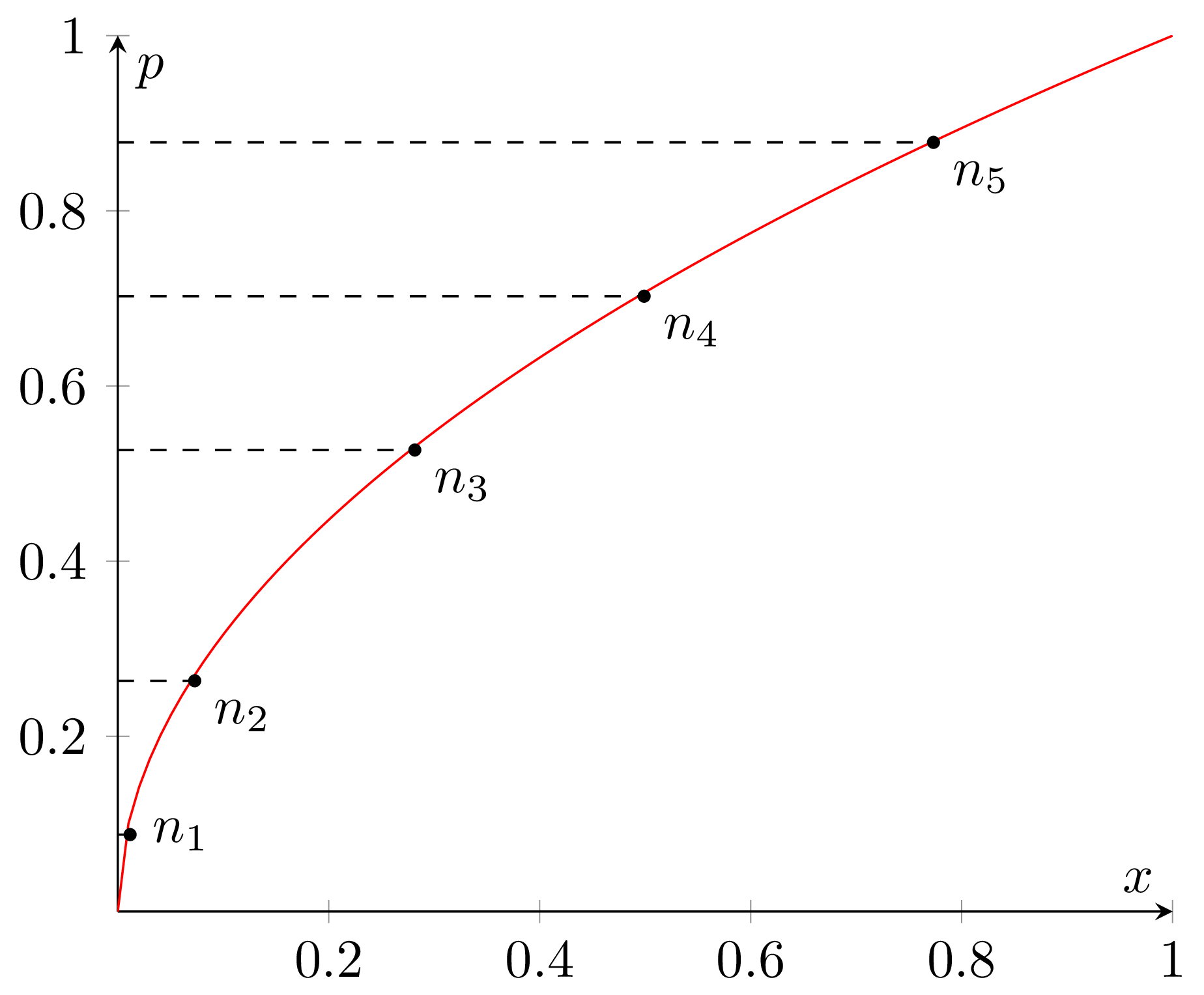
P2 is an interesting beast. To implement it we need to maintain a
small set of selected key points, or markers, from the data distribution.
Visually you can think of it as a sample cumulative distribution (the red line
on the graph below) with several points on it (n1 to n5).
Those points correspond to the selected quantiles, i.e. probabilities of the
sample X from the distribution being less than or equal to the corresponding
x coordinate, like on the following graph:
Audere est Facere, let’s try to implement it! In the following lines I’m going to show code snippets describing the main points of the algorithm, with the description of every snippet above the actual code. Here we’re going to keep everything:
data PSquare = PSquare
By everything I mean several things. First the quantile we need to estimate, which obviously should be within the interval (0, 1).
{ p :: Double
As I’ve mentioned we’re going to maintain a set of markers over the data we
get. Here is the current marker positions for the minimum observation, the
p/2, p, and (1+p)/2 quantiles. The positions are going to be
recalculated with every new observation we get.
, n :: !(Vector Int)
The current markers above represent current state of things, the quantile estimations, and can deviate from the ideal positions needed to calculate quantiles precisely. This means we would need to store those desired marker positions as well (also corresponding to the estimated quantile):
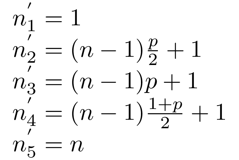
, ns :: !(Vector Double)
I’ve just realized I’m not sure how much is it helpful, but following the original paper we can also precompute increments for the desired marker positions we’re going to use later on:
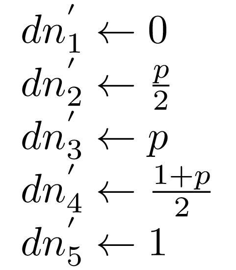
, dns :: !(Vector Double)
And the actual marker values, which are in fact the results of estimation, where:
-
q1 is the minimal observation
-
q2 is the estimate of
p/2quantile -
q3 is the estimate of
pquantile -
q4$ is the estimate of
(1+p)/2quantile
  , q :: !(Vector Double)

  }
  deriving (Show)
Essentially, with the data structure as above, to implement P2 algorithm we would need only two operations: add a new observation form the data stream and calculate the quantiles. To add a new observation we have to provide the P2 data structure and an observation value as arguments and return updated P2, for calculating the quantile estimation only P2 structure is enough:
class QuantileEstimator a where
    add :: a -> Double -> a
    quantile :: a -> Double
Now let’s implement them! The quantile calculation is dead simple, we simply need to return the second marker value, which, as you can recall, corresponds to the quantile we estimate:
instance QuantileEstimator PSquare where
  quantile ps@PSquare {..} = q ! 2
Now adding a new observation would be slightly harder. First we need to
accumulate at least 5 values to be able to initialize the data structure and
start the estimation process. As soon as there is enough values to start for
every new observation we need to remember it and recalculate the markers n
and corresponding values q.
  add !ps !value
    | V.length (q ps) < 4 = addNewValue ps value
    | V.length (q ps) == 4 = initPSquare $ addNewValue ps value
    | otherwise = updatePSquare ps value
    where
      addNewValue !ps@PSquare {..} !value = ps { q = V.snoc q value }
      initPSquare !ps@PSquare {..} = ps
        { q = V.fromList $ sort $ V.toList q
        , n = V.fromList $ [0..4]
        , ns = V.fromList $ [0, 2 * p, 4 * p, 2 + 2 * p, 4]
        , dns = V.fromList $ [0, p/2, p, (1 + p)/2, 1]
        }
      updatePSquare !ps !value =
        let
          !ps' = ps `insertObservation` value
          !qn' = adjustMarkers ps'
        in ps' { q = V.map fst qn'
               , n = V.map snd qn'
               }
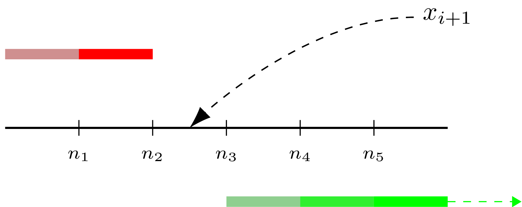
Let’s unwind this part. To remember a new observation means to add it to the observation set, but since P2 algorithm do not store it directly, such addition happens “virtually”. First we find to which interval between already estimated quantile values the new value (“x” on the following diagram) belongs to. Having this interval we now can update marker values if the new observation extends mininum/maximum boundaries. After than we need to “push” marker positions to the right of the found interval (the green arrow on the diagram shows which subset was shifted), representing a new element being inserted into the observation set.
Here is how we can implement it in a nutshell (I’ve omitted the nested functions):
insertObservation !ps@PSquare {..} !value =
  let
    !k = ps `findIntervalFor` value
    !newQ = ps `adjustIntervalsFor` value
    !newN = ps `incrementPositionFor` k
    !newNs = V.zipWith (+) ns dns
  in ps { n = newN, ns = newNs, q = newQ }
As the result we have the new data distribution which contains the new value. Thus, the “ideal” markers for this distribution are now different, and as the next step we need to reflect that. Essentially both position and height of the markers we maintain have to be corrected. For every one of the five markers we do the following:
adjustMarkers !ps@PSquare {..} = for (V.enumFromN 0 5) adjustMarkers'
  where
Nothing to do for the extreme markers q1, q5, they were already updated on the previous step.
    adjustMarkers' 0 = (q ! 0, n ! 0)
    adjustMarkers' 4 = (q ! 4, n ! 4)
For q2, q3, q4 find if they need to be shifted and in which direction. Note that the parabolic formula is being used here, we will get more details in a moment.
    adjustMarkers' i =
      let
        !d = (ns ! i) -. (n ! i)
        !direction = signum $ round d
        !qParabolic = parabolic ps i direction
The marker considered to be off the position if the distance from the ideal position is more than 1.
        !markerOff = (
             (d >= 1 && n ! (i + 1) - n ! i > 1) ||
             (d <= -1 && n ! (i - 1) - n ! i < -1))
If it’s indeed off the ideal place too much, recalculate the position and height.
        !n' = if markerOff
          then (n ! i) + direction
          else (n ! i)
        !q' = if markerOff
          then
For the algorithm to work the marker heights must always be in a non-decreasing order. If the parabolic formula we’ve calculated on the previous steps predict a value outside (qi-1, qi+1) interval, ignore it and use linear prediction.
            if (q ! (i - 1)) < qParabolic && qParabolic < (q ! (i + 1))
              then qParabolic
              else linear ps i direction
          else q ! i
      in (q', n')
I’ve already mentioned piecewise-parabolic function before, now let’s cover it with more details. We use P2 or piecewise-parabolic prediction formula to adjust marker heights after adding a new observation. The idea is to make the following assumption — whenever a marker ni is shifted to the side, its height follows the parabolic curve (as on the graph below) passing through any three adjacent markers qi = a n2i + b ni + c.
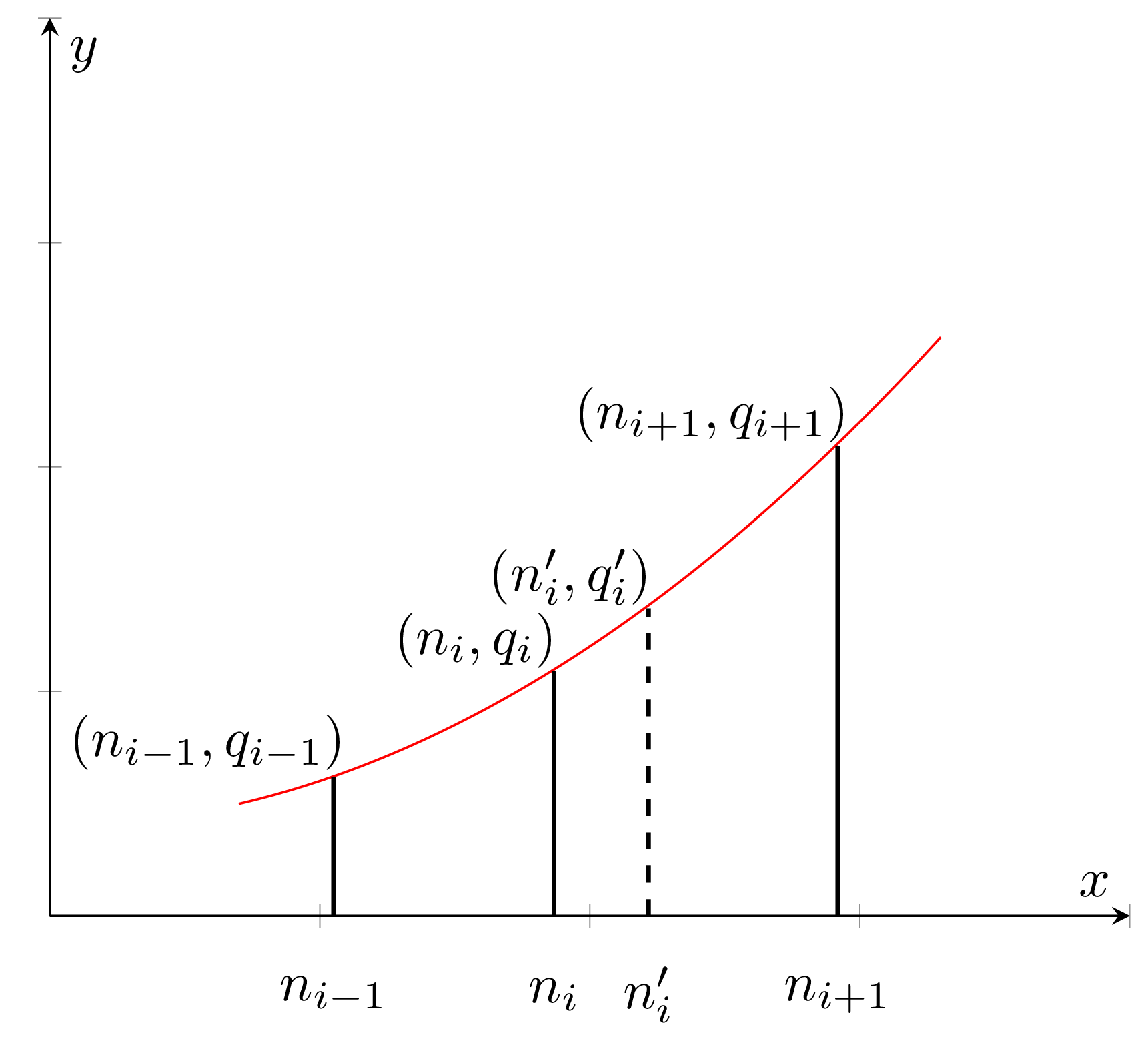
And the resulting formula for new height estimation is:
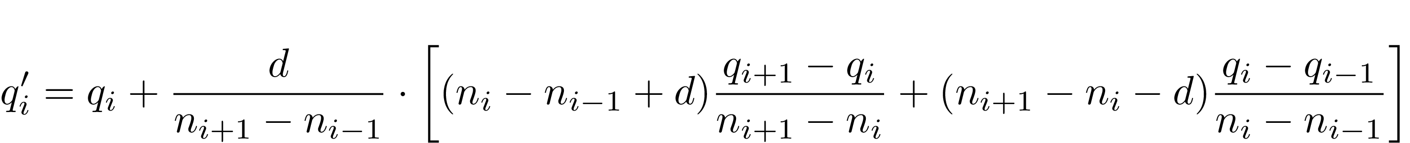
Now the implementation follows the formula, where i is number of the marker, d = ± 1 — direction taken from the previous computations.
parabolic :: PSquare -> Int -> Int -> Double
parabolic !ps@PSquare {..} i d =
    let
      !term1 = d ./. (n_i1 - n_i_1)
      !term2 = (n_i - n_i_1 + d) .* (q_i1 - q_i) /. (n_i1 - n_i)
      !term3 = (n_i1 - n_i - d) .* (q_i - q_i_1) /. (n_i - n_i_1)
    in
      q_i + term1 * (term2 + term3)
  where
    q_i = q ! i
    q_i1 = q ! (i + 1)
    q_i_1 = q ! (i - 1)
    n_i = n ! i
    n_i1 = n ! (i + 1)
    n_i_1 = n ! (i - 1)
And the same for the linear version, i — the number of marker, d = ± 1 — direction taken from previous computations.
linear :: PSquare -> Int -> Int -> Double
linear !ps@PSquare {..} i d =
  q_i + d .* (q_id - q_i) /. (n_id - n_i)
  where
    q_i = q ! i
    q_id = q ! (i + d)
    n_id = n ! (i + d)
    n_i = n ! i
Now that was more straightforward than I though.
3. Moving window
But what if we want to apply the same approach to estimate quantiles over a moving window? It’s not a void question, often we have to work with sliding intervals of data, either because the whole data set is too large, or we’re not interested in historical data. P2 do not really work well with streams of data, as shown in some more recent researches, and unfortunately I couldn’t find any published modifications to apply it in such fashion (if you know such examples, please let me know in the commentaries). It’s even understandable — the “virtual” nature of adding a new observation is one way process, and to maintain a window we would need to be able to somehow remove old observations. But still there are few options on the table.
In this blogpost the author suggests an interesting idea of using P2 as a black box and maintain over the data set two estimators at once, the active one (that’s where we’re currently adding observations) and the previous one. As soon as the current estimator have exactly one window of observations it becomes the previous, and we reset the current one to start from scratch.
In this way we always have two things at hand, the result of previous quantile estimation, and current estimations for the partial window. Imagine we have the data set, represented on the diagram below by the axis line, and currently we’re processing the element xn. We already know the quantile estimation E1 from the previous window, and current estimation E2 for part of the required window (shaded area on the diagram):
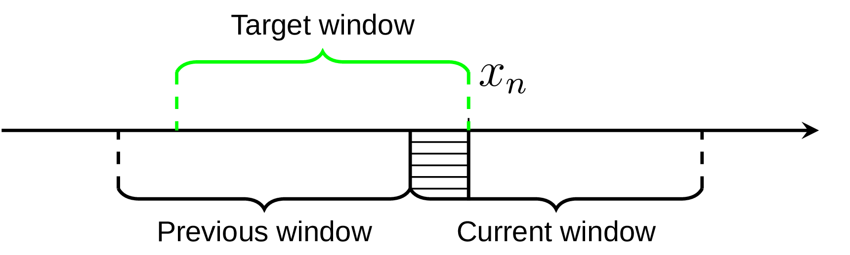
If the number of processed elements inside the current window is k and the window size is L, we could get reasonably good approximation for the target window using weighted sum:
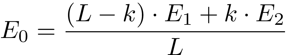
Of course this approach has its own downsides and provides less accuracy, especially around window borders, but overall works good.
I was pondering this idea for a while and came up with another variation of it that I find interesting. The core idea is same, we maintain two estimators over the data set, the previous and the current one. But after the switching to the current one (at the observation xk on the diagram) instead of keeping the previous one as static we still append new observations to it. In this way instead of the target window quantile estimation we get two estimations, one for the bigger window and one for the smaller window, as on the following diagram.
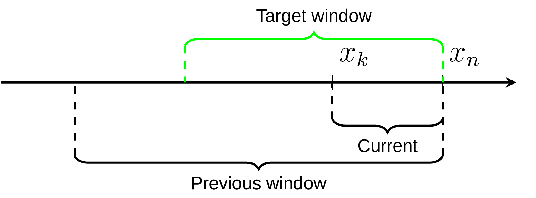
Assuming that the target window estimation should be somewhere in between, we can use the same weighted sum to get its approximation. Testing on the uniformly distributed data set shows only marginal difference from the original suggestion (the error median is only about 8% less) and in general this modified algorithm version requires more efforts to verify its accuracy. Andrey Akinshin has also proposed an idea that different window weights could be more optimal in this case (unfortunaty I haven’t got a chance yet to try it). But still I find both approaches show an interesting way of combining P2 estimators to achieve something new.
4. Is it practical yet?
To make it more down-to-earth experience we can look at the P2 algorithm from different perspectives. What do we need to be able to acquire practical knowledge and results from it?
Well, the most obvious thing is to be able to run it on different data distributions and under different conditions. For example, we can throw data generated by great statistics library at it. Another important aspect, which gets quite often forgotten on the way, is visualization. Unfortunately as human beings we’re not able to very efficiently interpret raw data. Even more, the representation is as much important as the data itself to draw correct conclusions. Fortunately for us, we’re backed by amazing Chart on this side. And the topic I personally find most exciting is performance, we need to analyze how fast or slow our algorithm is working and why. Criterion could be of great use for us in this area.
4.1 Accuracy
Let’s try it out! The original whitepaper contains interesting notes
about goodness of the P2 estimator with mean square errors, as well
as this blogpost demonstrates accuracy of the algorithm on
several distributions. My goal here would be somewhat simpler, I want to
compare the P2 algorithm with the
statistics package on the same data set. The
following graph shows the difference between P2 algorithm and the
quantile function with spss parameters (Weibull’s definition, corresponds
to method 6 in R and Mathematica) on uniformly distributed between (0, 1)
random data. Both approaches estimate 95th percentile of the data set. X axis
show the data set size (divided by 100, that’s why it’s referred to as
“scaled”), Y axis show the absolute difference between both:
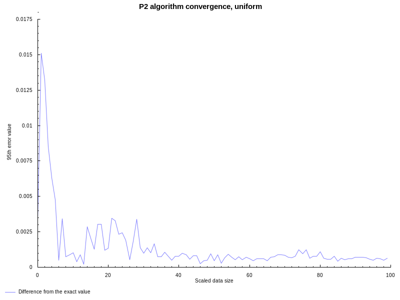
All good, like expected the P2 algorithm has noticeable error on smaller datasets, but accuracy improves with more and more observations available.
Now let’s experiment with moving version of P2. This time we’re
going to use normal distribution N(0,1), window size L = 100, and the goal
is to estimate median value. On the following graph you can see the results in
comparison with statistics package (all the parameters are the same as
before):
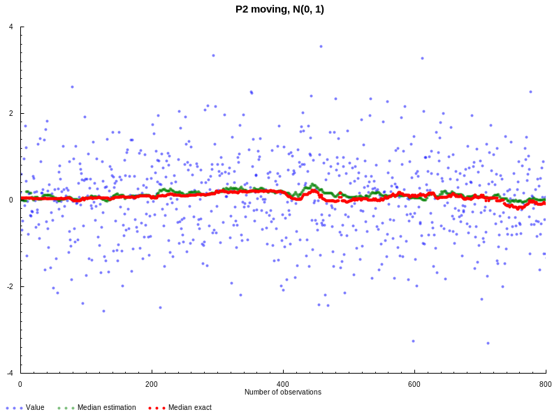
Doesn’t look bad, both quantile estimations are pretty close to each other. But
this example is probably not that interesting, because to actually verify the
moving nature we need to generate data with more variable quantiles. Following
suggestion from the original blogpost, lets generate sinusoidal
waves with noise and outliers. The window size is still the same L = 100, but
this time we estimate 95th percentile:
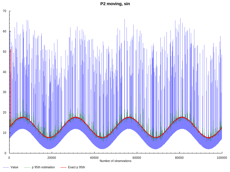
As we can see from the graph above, moving P2 is more affected by outliers, but still provides reasonably good estimation.
4.2 Measurement
How fast our implementation can work and how much data can we process within reasonable time? Are there any bottlenecks, why do they exist, and what could we do about them? We will see in a moment, but first we talk about how are we going to measure the performance. The algorithm is a pretty isolated thing, so we could just run it and see how much time does it take to finish. Could we?
The answer “it’s not that simple”, but fortunately for us most of the
complications could be handled by well known library criterion.
First this library will make it easy to benchmark pure functions, which could
be surprisingly tricky otherwise. If you try it directly without criterion,
laziness would ensure that we’d only do “real work” the first time through our
benchmarking loop. Another helpful thing criterion does is running our code
multiple times and reporting not the raw data, but benchmark statistics to help
understand if we got trustworthy results.
Now, let me show an example of what criterion could tell us:
time       76.65 ms   (76.00 ms .. 77.30 ms)
           1.000 R²   (0.999 R² .. 1.000 R²)
mean       77.05 ms   (76.44 ms .. 77.93 ms)
std dev    1.269 ms   (777.3 μs .. 2.014 ms)
The main column (first one from the left) represent most of the data we’re interested in:
-
time: estimates the time needed for a single execution of the activity using ordinary least-squares regression model. -
1.000 R²: R2 goodness-of-fit, shows how accurately the linear regression model fits the observed measurements, should lie between 0.99 and 1. -
mean,std dev: mean and standard deviation of execution time.
The following columns contains lower and upper bounds to the same values, measuring the accuracy of the main estimation using bootstrapping. There is a lot more to it, I can only encourage you to read the tutorial.
4.3 Variance
Even having nice statistical tools in place does not protect from data variance. Unfortunately we cannot test the algorithm implementation in vacuum, for whatever reason it has to run on a real hardware, full of noise and sometimes even steam. That’s why we have to make some efforts to get more repeatable and consistent results. I’ll limit this section to the very basics, as there is a nice writing about this topic. The basics are:
-
Have minimum unnecessary processes running simultaneously during the benchmark
-
Disable Intel Turbo
-
Disable HyperThreading
-
Set
scaling_governor -
Pin investigated process to one core
Those steps will not eliminate noise completely, but at least remove its most well-known sources.
5. Performance
Now it’s a right time to talk about speed, and we can start with setting up a
baseline for the analysis. Let’s run our algorithm implementation under
criterion on the data set of 105 values:
time       76.65 ms   (76.00 ms .. 77.30 ms)
           1.000 R²   (0.999 R² .. 1.000 R²)
mean       77.05 ms   (76.44 ms .. 77.93 ms)
std dev    1.269 ms   (777.3 μs .. 2.014 ms)
R2 indicated that the numbers are reasonably accurate. Is this fast enough? Could it be improved? We don’t know yet, so lets start digging in.
5.1 Language specific instrumentation and profiling
A language is not just words. It’s a culture, a tradition, a unification of a community, a whole history that creates what a community is. It’s all embodied in a language.
Noam Chomsky
Easiest first steps in every performance investigation could be done with tools
provided by the language ecosystem. As a simple example we could check
compilation options and see if we forgot something. In this case the code was
compiled using GHC-8.10.7 (and vector-0.12.3.0) with -O2
flag, which means “Apply every non-dangerous
optimization, even if it means significantly longer compile times”. I’ve also
tried to experiment with some other intriguingly sounding flags, like
-funbox-strict-fields -fspecialise-aggressively,
-funfolding-keeness-factor, or even use LLVM Code Generator, but got no
significant difference and not going into the details.
What I actually need to dive deeper into is modules. For simplicity I’ve
implemented everything, including the algorithm itself and testing
functionality, as a single module. Csaba Hruska noticed that this (totally
unintentionally from my side) results in better performance in comparison with
splitting some bits into different modules. For example separating PSquare,
MPSquare and benchmarking functionality makes the implementation slower,
apparently because the compiler can’t optimize across modules as efficiently as
withing a single module.
As soon as we’ve done with basic hygiene checks, we could start
profiling the code. To do this it has to be compiled with
-prof -fprof-auto (or add --profile flag into your stack build), and then
run it with +RTS -p. This will give us *.prof file, which unsurprisingly
contains profiling results. Profile can show us cost centres, how much
time was spent there and how much memory was allocated in it. Which is already
a lot of information to analyze!
First thing first. You’ve probably noticed I was using bang patterns everywhere I could in the code snippets above. That was my attempt to reduce thunks during computations, otherwise one could see GC being in the top of the cost centres:
COST CENTRE        MODULE                   %time %alloc

GC                 GC                        18.9    0.0
>>=                Data.Vector.Fusion.Util   15.6   19.4
It doesn’t really make sense to use lazy evaluation in this case, as everything
has to be calculated anyway. The same could be achieved with Strict and
StrictData pragmas, although there are still some subtleties I haven’t
investigated yet. Csaba Hruska also has tried more conventional approach with
the strict data types and no bang patterns, leaving it to the compiler
strictness analysis. The resulting implementation was not much slower.
With more strict code (and that was my starting point for benchmarking) the profile looks like this:
COST CENTRE        MODULE                   %time %alloc

>>=                Data.Vector.Fusion.Util  11.9   20.1
add.updatePSquare  Main                     10.0    7.5
basicUnsafeIndexM  Data.Vector.Primitive     8.1    9.3
I can imagine many of readers already noticed one potential and rather obvious
improvement even without looking at this profile. As it usually happens with
many high-level languages we use non-primitive data types in our
calculations. While more flexible, it also adds some overhead, which we could
avoid by using unboxed version of Vector. Let’s see how
much improvement could we get from this:
time       25.34 ms   (25.33 ms .. 25.36 ms)
           1.000 R²   (1.000 R² .. 1.000 R²)
mean       25.35 ms   (25.35 ms .. 25.35 ms)
std dev    8.172 μs   (4.901 μs .. 11.55 μs)
Yes, the dramatic difference, 25.34 ms vs 76.65 ms on 105 elements!
The profile above could also give you another interesting idea, somewhat
related to working at high/low level. In vector library documentation we
can notice that almost all operations are in fact safe operations. They do some
sanity checks, e.g. boundary checking or verifying if the vector is empty or
not. What will happen if we replace them with their unsafe counterpart, like
this?
get = V.unsafeIndex
update = V.unsafeUpd
Nothing easier than that, lets run criterion again, and indeed, few more
milliseconds have disappeared:
time       19.28 ms   (19.19 ms .. 19.41 ms)
           1.000 R²   (1.000 R² .. 1.000 R²)
mean       19.33 ms   (19.27 ms .. 19.52 ms)
std dev    238.9 μs   (73.03 μs .. 465.4 μs)
But we’re not done yet. So far we’ve replaced vectors with their unboxed version, but we still use boxed data types to compute parabolic and linear formulas. The most straightforward way to get rid of this as well is to unpack arguments we pass into the functions, perform necessary calculations, then pack the result back.
parabolic :: PSquare -> Int -> Double -> Double
parabolic !ps@PSquare {..} i (D# d) =
    let
      !term1 = d /## (n_i1 -## n_i_1)
      !term2 = (n_i -## n_i_1 +## d) *## (q_i1 -## q_i) /## (n_i1 -## n_i)
      !term3 = (n_i1 -## n_i -## d) *## (q_i -## q_i_1) /## (n_i -## n_i_1)
    in
      D# (q_i +## term1 *## (term2 +## term3))
  where
    (D# q_i) = q `get` i
    (D# q_i1) = q `get` (i + 1)
    (D# q_i_1) = q `get` (i - 1)
    (D# n_i) = n `get` i
    (D# n_i1) = n `get` (i + 1)
    (D# n_i_1) = n `get` (i - 1)
Looks a bit more cumbersome, but in this way we can shave off few more milliseconds:
time       16.85 ms   (16.75 ms .. 16.96 ms)
           1.000 R²   (1.000 R² .. 1.000 R²)
mean       16.88 ms   (16.82 ms .. 17.08 ms)
std dev    250.0 μs   (58.18 μs .. 495.4 μs)
Looks good, but now we face a challenge. As an input for the changes above we have used GHC profiling information with its pros and cons. Pros are obvious — it’s easy, but powerful, providing enough information to identify the largest bottlenecks, e.g. to avoid spending cycles doing unnecessary job. Cons are less noticeable from the first glance — this type of profiling information do not tell you why something is taking so much time.
5.2 Top-Down(ish) performance analysis
To find out which parts of our implementation are more time-consuming than expected we can apply Top-Down performance analysis. This methodology is explained in great details in Performance analysis and tuning on modern CPUS book and corresponding blog post as well. To summarize in a few words, following this approach it’s possible to analyze program performance in a “black box” manner. We need to collect specific metrics to classify the type of bottleneck we face, break it down to different levels and identify the responsible code. And there are even suitable tools for that!
Let’s start directly with perf. While it’s not the main purpose of it, perf
can provide first level breakdown of Top-Down approach. We just need to do some
preparations — our algorithm should run long enough. The following binary runs
P2 algorithm for a couple of minutes, but requires about 30 sec to
prepare the data for processing. Hence -D 30000 option to tell perf to wait
for 30000 milliseconds before starting collecting metrics (otherwise we will
collect metrics for an activity, which has nothing to do with the algorithm
itself).
$ perf stat -a --topdown -D 30000 -- taskset -c 0 ./PSquare

 Performance counter stats for 'system wide':

             retiring  bad speculation  frontend bound  backend bound
S0-D0-C0  1  64.7%             9.9%           13.3%          12.2%
It may sound a bit cryptic, so let’s do it step by step. As a reference we can take the diagram of Skylake Client Microarchitecture:
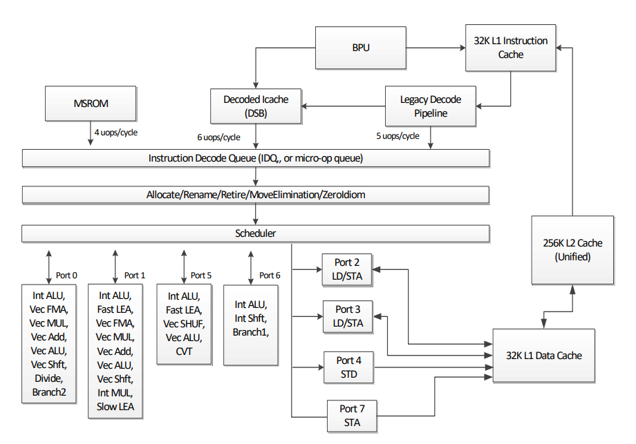
The Skylake core consists of an in-order front-end that fetches and decodes x86
instructions into a smaller uops and an 8-way
superscalar out-of-order backend. Top-Down approach talks using similar
vocabulary and replicates this structure. On the highest level there are few
types of bottlenecks (taken from pmu-tools, about it a bit later in more
details):
-
Backend bound: no uops are being delivered due to a lack of required resources for accepting new uops in the Backend. For example stalls due to data-cache misses or stalls due to the divider unit being overloaded are both categorized under Backend Bound.
-
Frontend bound: the processor’s Frontend undersupplies its Backend. For example stalls due to instruction-cache misses would be categorized under Frontend Bound.
-
Bad speculation: issued uops that do not eventually get retired, or the issue-pipeline was blocked due to recovery from earlier incorrect speculation. For example wasted work due to miss- predicted branches are categorized under Bad Speculation category.
-
Retired: this category represents fraction of slots utilized by useful work i.e. issued uops that eventually get retired. Ideally all pipeline slots would be attributed to the Retiring category. Retiring of 100% would indicate the maximum pipeline width throughput was achieved.
Having this in mind and looking at the numbers we’ve got everything looks pretty good. In fact before applying unboxed vector and following optimizations the fraction of frontend bound bottleneck was much higher. But we still could look deeper using pmu-tools.
To support Top-Down approach pmu-tools offers us a great tool
toplev. Using this tool we can break down potential
bottlenecks into more detailed levels and get more information. This comes with
couples of caveats though, the most important of which is probably
multiplexing. To give you an understanding what is it all about I need to
introduce a bit of context.
As many others, toplev uses CPU performance monitoring counters (PMC) to
collect necessary information. There is usually a fixed number of such
counters, and sometimes we want to collect more events than the available
number of counters. In this case the Linux kernel uses
multiplexing to give each event a chance to access the
monitoring hardware. This means an event is not measured all the time. At the
end of the run, the tool scales the count based on total time enabled vs time
running.
All this is done assuming we measure “steady” workload. As soon as workload
runs lots of different types of code in intervals less than the multiplex
interval, we get multiplexing errors. Fortunately we work with more or less
stable load produced by the P2 algorithm, and eventually I’ve disabled
multiplexing in toplev. Here is how it looks like:
$ toplev.py         \
    -D 30000        \   # delay, the same as for perf
    -l1             \   # first level of top-down
    --user          \   # measure only userspace
    --no-multiplex  \   # no multiplexing
    --verbose       \   # disregard threshold
    --perf          \   # show perf command
    --core C0 -- taskset -c 0 ./PSquare
I have to give one warning about verbose flag above. The thing is toplev
does not actually use the Top-Down thresholding mechanism when verbose is
enabled. Many TopDown nodes are only meaningful when their parent nodes crossed
their thresholds. That is why the section called “Top-Down(ish)”. As we’re
already working with relatively fast code, there are no huge bottlenecks and to
dive deeper I’ve enabled this mode.
When we run toplev on the first level, we get the numbers similar to perf.
This is encouraging, as it shows we’re on the right track, but we want more. It
will probably not bring any significant speed up, because as I’ve already said
bottlenecks are rather small, but it certainly could be exciting! With many
trials and errors — steering my way forward by filtering nodes via options
like --nodes '!+Backend_Bound.Core_Bound*/3' — I came to the conclusions that
the following types of events constitute the biggest part of all L1 Top-Down
categories:
-
Backend_Bound.Core_Bound.Ports_Utilization: This metric estimates fraction of cycles the CPU performance was potentially limited due to Core computation issues. Heavy data-dependency among contiguous instructions would manifest in this metric. Another example would be contention on some hardware execution unit other than Divider, e.g. when there are too many multiply operations.
-
Frontend_Bound.Fetch_Bandwidth.DSB: Represents Core fraction of cycles in which CPU was likely limited due to DSB (decoded uop cache) fetch pipeline. For example inefficient utilization of the DSB cache structure or bank conflict when reading from it.
-
Bad_Speculation.Branch_Mispredicts: Fraction of slots the CPU has wasted due to Branch Misprediction.
The first one, Ports_Utilization is somewhat expected. After all the
algorithm does fair share of computations estimating marker heights using
piecewise-parabolic formula. I don’t even think it would be easy to reduce this
further. But the rest of them — as small as they are — I found interesting.
Where are they coming from?
5.3 Searching for the explanations
Down and down into the deep
Who knows what we’ll find beneath?
Diamonds, rubies, gold, and more
Hidden in the mountain store
The first one has something to do with DSB, which is a HW unit called
Decoded Stream Buffer (do not mix it with DSB
barrier instruction) and essentially an uops cache. If an instruction is found
in DSB, there is no need to fetch it from memory, we feed the back-end with
already decoded uops. And as any cache it’s also a subject of cache misses,
which are coupled together with code alignment. Better aligned code could fit
into the less cache lines, thus causing less cache misses and producing more
efficient DSB usage.
Could that be the reason we see stumbled upon this using Top-Down approach? Unfortunately I don’t have a definitive answer to that question, but following the wiki page about block layout, GHC is indeed using somewhat simple algorithm to produce a block layout. There is apparently a room for improvement, as well as a room for getting worse.
Now what about the last one, branch misprediction? Following the toplev, the
baseline for this type currently is about %10 of slots that were stalled
becaues of branch misprediction:
BAD Bad_Speculation.Branch_Mispredicts % Slots 10.0 <
It’s probably not that much, but it gives a convenient ground for
investigation. To analyze what causes the stalls we need to sample
br_misp_retired.all_branches event. We could do it either manually, by
invoking perf, or leaving toplev to do it’s job via --run-sample option.
Unfortunately with high-level languages it’s only a half of the story, event
samples have to be somehow attributed to particular lines of code. You asking
how? Well, every time it depends…
Having debugging symbols in place I’ve found out a couple of hot spots in the
implementation. One of most significant ones was to my surprise the signum
function, used to identify in which direction to shift the markers. If you
replace it with some custom implementation it would be easier to identify,
otherwise GHC inlines stuff and leaves next to no traces about correlated lines
of code. For the sake of experiment I’ve applied NOINLINE pragma to avoid
that, and now the picture is more clear — the culprit leads us into the
internals with the specific implementation of the signum (the event
percentage below is 100%, which correspond only to this call site, overall it
constitutes about a half of the event samples in this test):
PSquare[42015d] 100.00 : 42015d: ja 42017f <base_GHCziFloat_zdfNumDoublezuzdcsignum_info+0x5f>]
Interesting, signum is quite branchy, is there anything to do about it? While
searching for some obvious solutions I’ve learned about possibility for
branchless implementation of many simple functions.
Overall it seems like a complicated topic and sometimes such branchless
approach could be beneficial, sometimes not. Let’s try it out in our case!
branchlessSignum :: Int -> Int
branchlessSignum !(I# x) = I# ((x ># 0#) -# (x <# 0#))
Now let’s test if the change will actually perform better or worse. First Top-Down metrics:
BAD Bad_Speculation.Branch_Mispredicts % Slots 5.1 <
An expected improvement, now less percent of slots are stalled on
misprediction. Unfortunately within the whole implementation it’s less visible
— testing this change with criterion will show some marginal, but stable
improvement of a fraction of millisecond as well:
time       16.55 ms   (16.48 ms .. 16.60 ms)
           1.000 R²   (1.000 R² .. 1.000 R²)
mean       16.59 ms   (16.56 ms .. 16.69 ms)
std dev    131.5 μs   (40.89 μs .. 255.6 μs)
Having this in mind I was curious about another bit of code. For every observation the algorithm needs to find out to which interval the observation belongs to. In the current implementation it boils down to many comparisons like:
location !ps@PSquare {..} !value
  | value < q `get` 0 = -1
  | value <= q `get` 1 = 0
  | value <= q `get` 2 = 1
  | value <= q `get` 3 = 2
  | value <= q `get` 4 = 3
  | value > q `get` 4 = 4
This construction is compiled into another hot spot of branches, visible in
perf annotate result. Not only there are many branches inside, it also does
not take into account likeness/unlikeness of some particular values — over the
time one can expect only minority of all the observation will belong to the
extreme intervals. Is it possible to avoid this?
Well, GHC by itself doesn’t yet provide control over branch prediction. But probably it’s possible to squeeze out some more milliseconds by replacing it with some C via FFI? In the replacement function we could tell GCC more about which values we expect more often, and use SIMD instructions to perform more comparisons at once. Oh, what the heck, lets try it out as well!
I’ve ended up with the following implementation:
import Data.Coerce (coerce)

foreign import ccall unsafe "location" c_location :: CDouble
                                                  -> Ptr CDouble
                                                  -> CInt

location !ps@PSquare {..} !value =
  let
    !(qFPtr, qLen) = V.unsafeToForeignPtr0 q
    !qPtr = unsafeForeignPtrToPtr qFPtr
    !loc = (coerce c_location) value qPtr :: CInt
    !result = fromIntegral loc
  in result
Here we call C implementation of location function and pass vector data via
pointer. But it’s not that simple as it looks like, there is always a trick.
To make this work we have to use Storable version of vectors instead
Unboxed, otherwise data will be stored in GC-managed unpinned memory and
garbage collector is free to move it around. This is of course an issue if we
want to share data via FFI, and to prevent that is exactly the goal of
Storable. Using it data will be stored in pinned memory and could be share.
The downside is more memory fragmentation and corresponding performance
overhead. Now lets take a look at the C counterpart:
#include <immintrin.h>
#include <stdio.h>

#define unlikely(x)     __builtin_expect((x),0)

int location(const double value, const double *vector)
{
	__m256d simd_vec = _mm256_loadu_pd(vector + 1);
	__m256d values = _mm256_set_pd(value, value, value, value);
	__m256d cmp;

	if (unlikely(value < vector[0]))
		return -1;

	if (unlikely(value > vector[4]))
		return 4;

	// Compare 4 elements, vector[1..4]
	cmp = _mm256_cmp_pd(values, simd_vec, _MM_CMPINT_LE);
	return __builtin_ctz(_mm256_movemask_pd(cmp));
}
The function has only two arguments: value represents the new observation and
vector corresponds to the storable vector of marker heights. Inside we tell
the compiler that two less than/greater than comparison are less likely than
everything else. The rest is to compare with less than or equal operator four
pairs of values. This fits nicely to SIMD instruction _m256_cmp_pd, which can
compare four double precision values at once and return comparison mask as the
result. The only thing left is to find out the first non-zero index in the mask
and it’s done. At it even works!
But as soon as we try to get criterion numbers it will be disappointingly
slow. The first possible explanation I’ve discovered was GHC will not inline C
implementation. If you’ve compiled everything with the debugging symbols (which
I encourage you to do), you’ll see something like this:
$ objdump -l -D PSquare
  ...
PSquare.lhs:163
  ...
  4135b3:   e8 28 2a 00 00    callq  415fe0 <location>
  ...

0000000000415fe0 <location>: location(): location.c:17
  ...
_mm256_cmp_pd(): include/avxintrin.h:398
  416000:   c5 f5 c2 cb 02    vcmplepd %ymm3,%ymm1,%ymm1
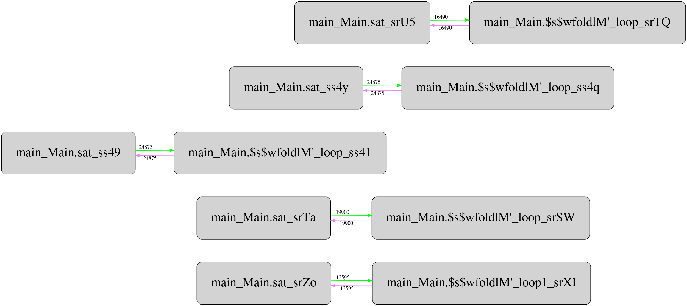
But it turns out there is a twist. Csaba Hruska did more extensive investigation using GHC Whole Program Compiler and exported the corresponding intermediate representation (STG IR) for analyze. He has got pretty strange runtime call graphs, which after filtering the most frequent calls looks like this for the original “unboxed” version:
And this is the same for stored version:
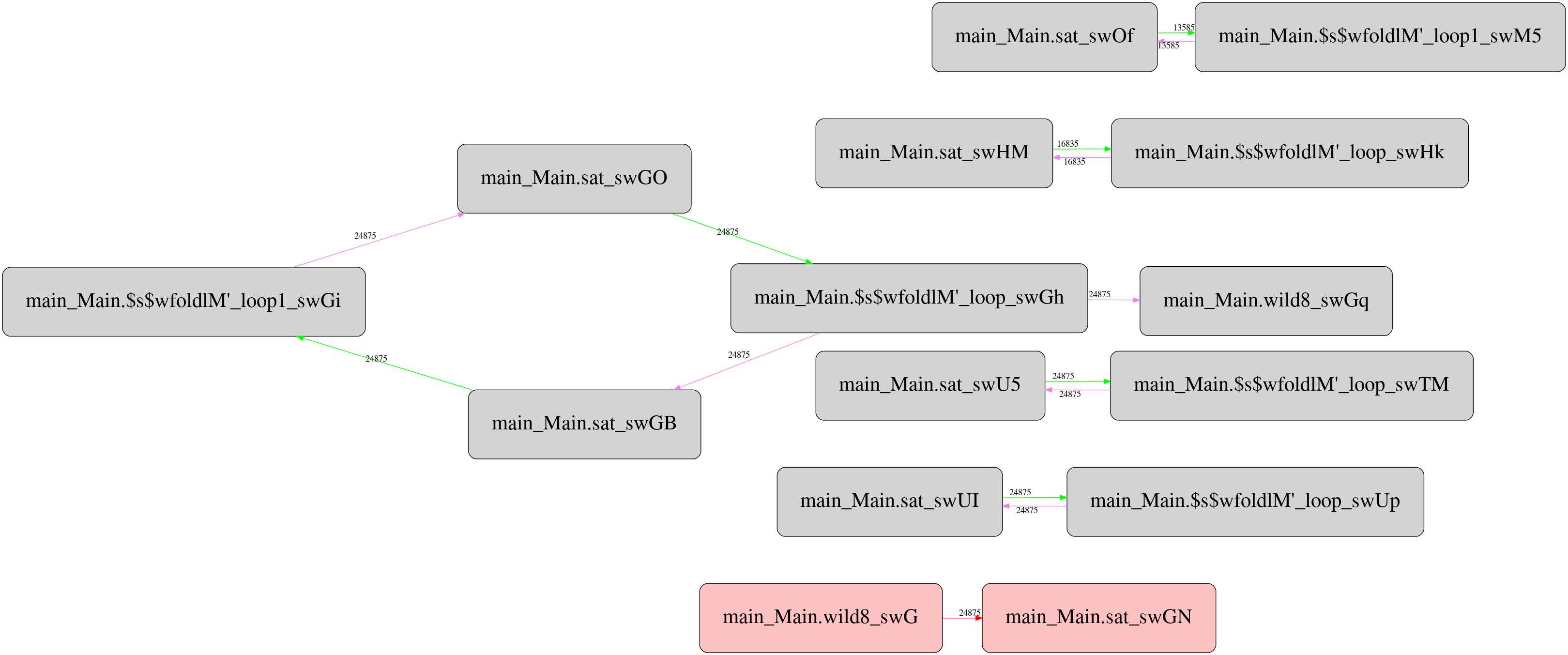
Not only it’s more complex than the original one, it contains one mysterious
call with unknown call site type (boxes highlighted with red) that reads
Double values from the storable vector. It seems the call appears only in
storable version, and located between two criterion_getcputime FFI calls. I
haven’t investigated yet what this call does and why, but maybe someone from
the readers can suggest potential explanation.
I’ve put the final version of implementation here. In case if you have
interesting ideas for improvements or commentaries, feel free to share. As I
was concentrating on the algorithm, everything was simply build with
nix-shell and ghcWithPackages.
6. Final thoughts
So far we’ve covered quantile estimation from many sides. But there is obviously much more to it than I could sum up in this blog post! Much more math and interesting algorithms, much more cool compiler stuff and performance analysis tricks. And the synergy of those topics brings unexpectedly pragmatic perspective if you want to apply such knowledge.
I hope with this writing I’ve managed to inspire someone and to give necessary instruments to do great things.
Acknowlegements
Thanks a lot to Csaba Hruska (@csaba_hruska), Andrey Akinshin (@andrey_akinshin) and Denis Bakhvalov (@dendibakh) for review and commentaries!
References
1. Arandjelović, Ognjen, Duc-Son Pham, and Svetha Venkatesh. “Two maximum entropy-based algorithms for running quantile estimation in nonstationary data streams.” IEEE Transactions on circuits and systems for video technology 25.9 (2014): 1469-1479.
2. Munro, J. Ian, and Mike S. Paterson. “Selection and sorting with limited storage.” Theoretical computer science 12.3 (1980): 315-323.
3. Hyndman, Rob J.; Fan, Yanan (November 1996). “Sample Quantiles in Statistical Packages”. American Statistician. American Statistical Association. 50 (4): 361–365. doi:10.2307/2684934.
4. Jain, Raj, and Imrich Chlamtac. “The P² algorithm for dynamic calculation of quantiles and histograms without storing observations.” Communications of the ACM 28, no. 10 (1985): 1076-1085.
5. Schmeiser BW, Deutsch SJ. Quantile estimation from grouped data: The cell midpoint. Communications in Statistics-Simulation and Computation. 1977 Jan 1;6(3):221-34.